Download

1 / 44
440 likes | 444 Views
This study presents the methodology for analyzing long-term tidal forcings and mapping and analyzing marsh conditions and changes in Delaware's Inland Bays. Preliminary results for the years 1992 and 2007 are provided, along with challenges and limitations of the methodology.

E N D
METHODS FOR QUANTIFYING TIDAL WETLAND CHANGES IN DELAWARE’S INLAND BAYS (1937 to 2007) Andrew Homsey, Richard T. Field, Jo Young-Heon, Geri Pepe, Kurt Philipp 2 February, 2011
Introduction Project undertaken with DE Center for Inland Bays, UD CEOE Acreage and Condition Trends for Marshes of Delaware’s Inland Bays as an Environmental Indicator and Management Tool Y. H. Jo, K. R. Philipp, R. T. Field, G. Pepe, and A.R. Homsey USEPA Applied Research Efforts (RARE) Grant Through Center for the Inland Bays (Chris Bason) Coordinated with DNREC personnel
Introduction First year of a three year project Two main parts Long-term tidal analysis to analyze major tidal forcings in the Inland Bays Historic mapping and analysis of marsh conditions and changes over time (1937, 1968, 1992, 2007)
Introduction Presented are preliminary results. Details only for the latter two dates (1992, 2007), which have comprehensive supporting data Focus will be on the development of the methodology to assess changes, including challenges and limitations
Study Area Inland Bays of Delaware, including Rehoboth Bay Indian River Bay Little Assawoman Bay (DE portion) Study focus Estuarine wetlands plus contiguous non-tidal wetlands 300 m buffer inland to assess contiguous upland conditions and changes
Project Scope • Tidal analysis • Based on Lewes continuous NOAA tidal gauge and several shorter-term USGS tidal stations in the Bays • Need to model the lag due to inlet constriction • Based on the tide record, isolate various long-term forcings • NAO, metonic (~18.6 yr. lunar) cycle, El Nino, La Nina • Isolates the effect of SLR • Allows us to determine RSL at time of historic imagery, and in the future.
Project Scope • Tidal analysis
Project Scope • Data needs for historic condition mapping and change analysis • Imagery • 2007, 1992, 1968, 1937 • Pre-process as necessary • Use of TIFs to allow false-color IR
Project Scope • Supporting datasets • 1992 SWMP, 2009 SWMP/NWI • 1992 and 2007 LULC • High marsh from NVCS (Robert Coxe/DNREC), • Other supporting info (e.g., Daiber wetlands maps)
Project Scope • Initial tasks • Work out procedures/work flow • What metrics are important, and how best to capture them • Quality Assurance Plan • Generate data models, processing software, derived data sets
Project Scope • Training and Fieldwork • Photo interpretation of modern and historical imagery requires training (possible student in upcoming year) • Site visit with CIB and EPA
Project Scope • Potential uses • Project described generates information to be used in subsequent analysis, not looking at causes of change • Can be used to guide future research and management/policy decisions and directions
Project Scope • Potential uses • Monitor SWD • Assess effects of RSLR • Identify potential for “strategic retreat” • Track shoreline migration • Quantify wetland loss, land cover conversion and buffer condition, • Anticipate, guide, and plan for future changes
Workflow/Data Details • Use 1992 and 2007/9 DE wetlands data as basis • For upland information, use LULC layers • Derive data layers from SWMP • Generate an aggregating unit on which to summarize marsh metrics • 60 m grid chosen after experimentation
Workflow/Data Details • Wetlands • Use SWMP data and pre-release of new NWI • For 1992, need to fill in Assawoman gap using reinterpretation of 2007 data • Uplands • Use official Delaware framework layers
Workflow/Data Details • Shoreline • Edit SWMP to exclude boat basins and marsh channels • Upland line – Border between estuarine wetland and upland • Same process for 1992 and 2007 • Comparison across years will determine transgression/deterioration
Workflow/Data Details • Offshore baseline • Shoreline/upland transects • Intended to be used to quantify changes • Problems include definition of shoreline, sinuosity and fragmentation
Workflow/Data Details • Other key features captured with 6m raster layers • Areas along upland/wetland boundary which are hardened (limit migration) • Areas within marsh with open water/mudflats/salt pannes • These layers are “painted” using image processing tools.
Workflow/Data Details • Presence of ditching • Historically, ditching for mosquito control and salt hay drainage has affected much if not most of DE’s salt marshes • Excavation • Indicates areas of human agency
Workflow/Data Details • Merged land cover dataset • SWMP + LULC (+ NVCS) • Consistent classification scheme • In particular, capture the many types of in-marsh open water areas. Need to distinguish natural from human changes.
Workflow/Data Details • Attribution and Delineation • Some degree of crosswalk, but a good deal of heads-up analysis • Hardening and open water marsh areas require tile-by-tile analysis • Many software tools were developed to assist (attribution, photo tile controls, cross-tabulation)
Workflow/Data Details • Once consistent data layers created • Rasterization • Cross-tabulation of areas • Generation of tabular summaries, linked back to the aggregation grid • Spreadsheet manipulation
Preliminary Results • Hardening and Open Water Analysis • 2007 only • Results of “painting” summarized across aggregation grid
Preliminary Results • Marsh Changes, 1992 – 2007
Special thanks to • Richard Field, Jo Young, Kurt Philipp, Geri Pepe • Chris Bason, CIB • Robert Coxe, DNREC • Mark Biddle, Amy Jacobs, DNREC • Vic Klemas, UD Center for Remote Sensing • USEPA