Download
1 / 25
260 likes | 275 Views
Image Compression -- JPEG. Instructor: L. J. Wang, Dept. of Information Technology, National Pingtung Institue of Commerce Reference: Mark S. Drew, Simon Fraser University, Canada. (http://www.sfu.ca/)

E N D
Image Compression -- JPEG Instructor: L. J. Wang, Dept. of Information Technology, National Pingtung Institue of CommerceReference: Mark S. Drew, Simon Fraser University, Canada. (http://www.sfu.ca/) Reference: W.B. Pennebaker, J.L. Mitchell, "The JPEG Still Image Data Compression Standard", Van Nostrand Reinhold, 1993. L. J. Wang
What is JPEG? • "Joint Photographic Expert Group". Voted as international standard in 1992. • Works with color and grayscale images. • Motivation • The compression ratio of lossless methods (e.g., Huffman, Arithmetic, LZW) is not high enough for image and video compression, especially when the distribution of pixel values is relatively flat. • JPEG uses transform coding, it is largely based on the following observations: • A large majority of useful image contents change relatively slowly across images, i.e., it is unusual for intensity values to alter up and down several times in a small area, for example, within an 8 x 8 image block. Translate this into the spatial frequency domain, it says that, generally, lower spatial frequency components contain more information than the high frequency components which often correspond to less useful details and noises. • Pshchophysical experiments suggest that humans are more receptive to the loss of higher spatial frequency components than the loss of lower frequency components. L. J. Wang
JPEG overview • Encoding • Decoding -- Reverse the order L. J. Wang
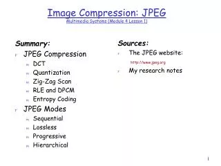
Major Steps for JPEG • DCT (Discrete Cosine Transformation) • Quantization • Zigzag Scan • DPCM on DC component • RLE on AC Components • Entropy Coding L. J. Wang
1. Discrete Cosine Transform (DCT) • From spatial domain to frequency domain: • f(i,j) → F(u,v) • DEFINITIONS L. J. Wang
2. Quantization • F'[u, v] = round ( F[u, v] / q[u, v] ). • Why? -- To reduce number of bits per sample • Example: 101101 = 45 (6 bits). q[u, v] = 4 --> Truncate to 4 bits: 1011 = 11. • Quantization error is the main source of the Lossy Compression. • Uniform Quantization • Each F[u,v] is divided by the same constant N. • Non-uniform Quantization -- Quantization Tables • Eye is most sensitive to low frequencies (upper left corner), less sensitive to high frequencies (lower right corner) • The Luminance Quantization Table q(u, v) • The Chrominance Quantization Table q(u, v) • The numbers in the above quantization tables can be scaled up (or down) to adjust the so called quality factor. • Custom quantization tables can also be put in image/scan header. L. J. Wang
2. Quantization (II) L. J. Wang
3. Zig-zag Scan • Why? -- to group low frequency coefficients in top of vector. • Maps 8 x 8 to a 1 x 64 vector L. J. Wang
4. Differential Pulse Code Modulation (DPCM) on DC component • DC component is large and varied, but often close to previous value. • Encode the difference from previous 8 x 8 blocks -- DPCM L. J. Wang
5. Run Length Encode (RLE) on AC components • 1 x 64 vector has lots of zeros in it. • Keeps skip and value, where skip is the number of zeros and value is the next non-zero component. • Send (0,0) as end-of-block sentinel value. L. J. Wang
6. Entropy Coding • Categorize DC values into SIZE (number of bits needed to represent) and actual bits. • Example: if DC value is 4, 3 bits are needed. • Send off SIZE as Huffman symbol, followed by actual 3 bits. L. J. Wang
6. Entropy Coding (II) • For AC components two symbols are used: Symbol_1: (skip, SIZE), Symbol_2: actual bits. Symbol_1 (skip, SIZE) is encoded using the Huffman coding, Symbol_2 is not encoded. • Huffman Tables can be custom (sent in header) or default. L. J. Wang
JPEG Bitstream L. J. Wang
JPEG Bitstream (II) • A "Frame" is a picture, a "scan" is a pass through the pixels (e.g., the red component), a "segment" is a group of blocks, a "block" is an 8 x 8 group of pixels. • Frame header: sample precision (width, height) of image number of components unique ID (for each component) horizontal/vertical sampling factors (for each component) quantization table to use (for each component) • Scan header Number of components in scan component ID (for each component) Huffman table for each component (for each component) L. J. Wang
JPEG Bitstream (III) • Misc. (can occur between headers) Quantization tables Huffman Tables Arithmetic Coding Tables Comments Application Data L. J. Wang
Four JPEG Modes • Sequential Mode • Lossless Mode • Progressive Mode • Hierarchical Mode ** In "Motion JPEG", Sequential JPEG is applied to each image in a video. L. J. Wang
1. Sequential Mode • Each image component is encoded in a single left-to-right, top-to-bottom scan. • Baseline Sequential Mode, the one that we described above, is a simple case of the Sequential mode: • It supports only 8-bit images (not 12-bit images) • It uses only Huffman coding (not Arithmetic coding) L. J. Wang
2. Lossless Mode • A special case of the JPEG where indeed there is no loss. Its block diagram is as below: L. J. Wang
2. Lossless Mode (II) • It does not use DCT-based method! Instead, it uses a predictive (differential coding) method: • A predictor combines the values of up to three neighboring pixels (not blocks as in the Sequential mode) as the predicted value for the current pixel, indicated by "X" in the figure below. The encoder then compares this prediction with the actual pixel value at the position "X", and encodes the difference (prediction residual) losslessly. L. J. Wang
2. Lossless Mode (III) • It can use any one of the following seven predictors : • Since it uses only previously encoded neighbors, the very first pixel I(0, 0) will have to use itself. Other pixels at the first row always use P1, at the first column always use P2. L. J. Wang
2. Lossless Mode (IV) • Effect of Predictor (test result with 20 images): • Note: "2D" predictors (4-7) always do better than "1D" predictors. L. J. Wang
2. Lossless Mode (V) • Comparison with Other Lossless Compression Programs (compression ratio): L. J. Wang
3. Progressive Mode • Goal: display low quality image and successively improve. • Two ways to successively improve image: • Spectral selection: Send DC component and first few AC coefficients first, then gradually some more ACs. • Successive approximation: send DCT coefficients MSB (most significant bit) to LSB (least significant bit). (Effectively, it is sending quantized DCT coefficients frist, and then the difference between the quantized and the non-quantized coefficients with finer quantization stepsize.) L. J. Wang
4. Hierarchical Mode • A Three-level Hierarchical JPEG Encoder (From V. Bhaskaran and K. Konstantinides, "Image and Video Compression Standards: Algorithms and Architectures", 2nd ed., Kluwer Academic Publishers, 1997.) • (a) Down-sample by factors of 2 in each dimension, e.g., reduce 640 x 480 to 320 x 240 • (b) Code smaller image using another JPEG mode (Progressive, Sequential, or Lossless). • (c) Decode and up-sample encoded image • (d) Encode difference between the up-sampled and the original using Progressive, Sequential, or Lossless. • Can be repeated multiple times. • Good for viewing high resolution image on low resolution display. L. J. Wang
4. Hierarchical Mode (II) L. J. Wang