Download
1 / 16
230 likes | 600 Views
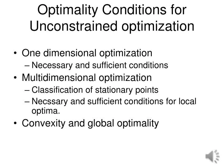
Optimality Conditions for Unconstrained optimization. One dimensional optimization Necessary and sufficient conditions Multidimensional optimization Classification of stationary points Necssary and sufficient conditions for local optima. Convexity and global optimality.

E N D
Optimality Conditions for Unconstrained optimization • One dimensional optimization • Necessary and sufficient conditions • Multidimensional optimization • Classification of stationary points • Necssary and sufficient conditions for local optima. • Convexity and global optimality
One dimensional optimization • We are accustomed to think that if f(x) has a minimum then f’(x)=0 but….
1D Optimization jargon • A point with zero derivative is a stationary point. • x=5, Can be a minimum A maximum An inflection point
Optimality criteria for smooth 1D functions at point x* • f’(x*)=0 is the condition for stationarity and a necessary condition for a minimum or a maximum. • f“(x*)>0 is sufficient for a minimum • f“(x*)<0 is sufficient for a maximum • With f”(x*)=0 needs information from higher derivatives. • Example?
Problems 1D • Classify the stationary points of the following functions from the optimality conditions, then check by plotting them • 2x3+3x2 • 3x4+4x3-12x2 • x5 • f=x4+4x3+6x2+4x • Answer true or false: • A function can have a negative value at its maximum point. • If a constant is added to a function, the location of its minimum point can change. • If the curvature of a function is negative at a stationary point, then the point is a maximum.
Taylor series expansion in n dimensions • Expanding about a candidate minimum x* • This is the condition for stationarity
Conditions for minimum • Sufficient condition for a minimum is that • That is, the matrix of second derivatives (Hessian) is positive definite • Simplest way to check positive definiteness is eigenvalues: All eigenvalues need to be positive • Necessary conditions matrix is positive-semi definite, all eigenvalues non-negative
Types of stationary points • Positive definite: Minimum • Positive semi-definite: possibly minimum • Indefinite: Saddle point • Negative semi-definite: possibly maximum • Negative definite: maximum
Problems n-dimensional • Find the stationary points of the following functions and classify them:
Global optimization • The function x+sin(2x)
Convex function • A straight line connecting two points will not dip below the function graph. • Convex function will have a single minimum. Sufficient condition: Positive semi-definite Hessian everywhere.
Problems convexity • Check for convexity the following functions. If the function is not convex everywhere, check its domain of convexity.
Reciprocal approximation • Reciprocal approximation (linear in one over the variables) is desirable in many cases because it captures decreasing returns behavior. • Linear approximation • Reciprocal approximation
Conservative-convex approximation • At times we benefit from conservative approximations • All second derivatives of fC are non-negative • Called convex linearization (CONLIN), Claude Fleury
Problems approximations • Construct the linear, reciprocal, and convex approximation at (1,1) to the function • Plot and compare the function and the two approximations. • Check on their properties of convexity and conservativeness.