One-Dimensional Unconstrained Optimization Chapter 13

1. One-Dimensional Unconstrained OptimizationChapter 13 Credit: Prof. Lale Yurttas, Chemical Eng., Texas A&M University

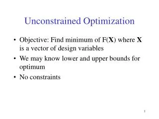
2. Mathematical Background • An optimizationor mathematical programming problem is generally stated as: Find x, which minimizes or maximizesf(x)subject to Where x is an n-dimensional design vector, f(x) is the objective function, di(x) are inequality constraints, ei(x) are equality constraints, and ai and bi are constants • Optimization problems can be classified on the basis of the form of f(x): • If f(x) and the constraints are linear, we have linear programming. • If f(x) is quadratic and the constraints are linear, • we have quadratic programming. • If f(x) is not linear or quadratic and/or the constraints are nonlinear, we have nonlinear programming. • When equations(*) are included, we have a constrained optimization problem; otherwise, it is unconstrained optimization problem.

3. One-Dimensional Unconstrained Optimization • Root finding and optimization are related. Both involve guessing and searching for a point on a function. Difference is: • Root finding is searching for zeros of a function • Optimization is finding the minimum or the maximum of a function of several variables. • In multimodal functions, both local and global optima can occur. We are mostly interested in finding the absolute highest or lowest value of a function. • How do we look for the global optimum? • By graphing to gain insight into the behavior of the function. • Using randomly generated starting guesses and picking the largest of the optima • Perturbing the starting point to see if the routine returns a better point

4. Golden Ratio • A unimodal function has a single maximum or a minimum in the a given interval. For a unimodal function: • First pick two points that will bracket your extremum [xl, xu]. • Then, pick two more points within this interval to determine whether a maximum has occurred within the first three or last three points Golden Ratio

5. Golden Ratio The Parthenon in Athens, Greece was constructed in the 5th century B.C. Its front dimensions can be fit exactly within a golden rectangle

6. Golden-Section Search • Pick two initial guesses, xl and xu, that bracket one local extremum of f(x): • Choose two interior points x1 and x2 according to the golden ratio Evaluate the function at x1 and x2 : • If f(x1) > f(x2) then the domain of x to the left of x2 (from xlto x2) does not contain the maximum and can be eliminated. Then, x2 becomes the new xl • If f(x2) > f(x1), then the domain of x to the right of x1 (from x1to xu) can be eliminated. In this case, x1 becomes the new xu. • The benefit of using golden ratio is that we do not need to recalculate all the function values in the next iteration. If f(x1) > f(x2) then Newx2 x1else Newx1  x2 Stopping Criteria | xu - xl | < e

7. Fig 13.5

8. Finding maximum through Quadratic Interpolation • If we have 3 points that jointly bracket a maximum (or minimum), then: • Fit a parabola to 3 points (using Lagrange approach) and find f(x) • Then solve df/dx = 0 to find the optimum point.

9. Example (from the textbook): Use the Golden-section search to find the maximum of f(x) = 2 sinx – x2/10 within the interval xl=0 and xu=4

10. Newton’s Method • A similar approach to Newton- Raphson method can be used to find an optimum of f(x) by finding the root of f’(x) (i.e. solving f’(x)=0): • Disadvantage: it may be divergent • If it is difficult to find f’(x) and f”(x) analytically, then a secant-like version of Newton’s technique can be developed by using finite-difference approximations for the derivatives.

11. Example 13.3: Use Newton’s method to find the maximum of f(x) = 2 sinx – x2/10 with an initial guess of x0 = 2.5 Solution: