Interannual Long Equatorial Waves in the Tropical Atlantic (1981-2000)

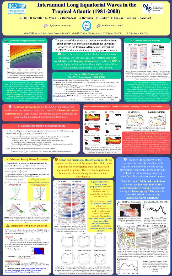
1. SLA Comparison at 0°N RMS (BL ZCA) ZCA Comparison at 0°N 28.875°N 5.875°N 0°N 3.125°S 28.875°S 50°W 36°W 16°W 10°E 20°E Interannual Long Equatorial Waves in the Tropical Atlantic (1981-2000) S. Illig 1, B. Dewitte 1, N. Ayoub 1 , Y DuPenhoat 1, G. Reverdin 2, P. DeMey 1 , F. Bonjean3 , and G.S.E. Lagerloef3 illig@notos.cst.cnes.fr bxd@notos.cst.cnes.fr (1)LEGOS, 14 av. E. Belin, 31400 Toulouse, FRANCE (2) LODYC, Case 100, 4 pl Jussieu, 75252 Paris, FRANCE (3) ESR, Seattle, WA, USA The purpose of this study is to determine to which extent linear theory can explain the interannual variability observed in the Tropical Atlantic and interpret the TOPEX/Poseidon data in terms of long equatorial waves. CLIPPER Interannual Anomalies CLIPPER Mean Temperature Vertical Structure  Due to the relative scarcity of observed data in the subsurface, we first investigate the vertical structure variability in the Tropical Atlantic based on the CLIPPER project high-resolution Ocean General Circulation Model (OGCM) simulation for the 1981-2000 period. Figure 2: Hovmuller representation of Sea level Anomalies (SLA) from T/P+ ERS and CLIPPER along the equator. Map of RMS Bonjean & Lagerloef (BL) satellite currents (to be compared to Fig. 3a). Plots of correlation (black) and RMS difference (red) along the equator between observed and simulated SLA/ZCA. Interannual anomalies are estimated relative to the climatology over the 1993-1999 period. Units are cm and cm/s respectively. Figure 1: Mean vertical structure temperature along the equator from CLIPPER (1981-1999). The mean isotherms 16°C, 20°C and 24°C are represented in black lines for the simulation and in white line for the TAOSTA observations (Vauclair and Du-Penhoat, 2001). Unit is °C. 1. The CLIPPER SIMULATION The ATL6 Experiment (1980-2000) Numerical model:OPA Ocean General Circulation Model v. 8.2(Madec et al, 1998) : • This simulation was performed for the CLIPPER Project (Barnier et al. 2001) and kindly provided to us by the CLIPPER project team. • Domain : Longitudes :98.5°W-0°E - Latitudes :75°S-70°N, with realistic coastline and bathymetry. • Resolution :  Zonal resolution = 1/6°,  Meridional resolution varies from 4.8km near the poles to 18.5km at the equator,  Vertical resolution = 42 levels(which 14  first 300 m). • Viscosity and vertical diffusivity : TKE model (Blanke and Delecluse, 1993). Atmospheric forcingECWMF (daily fields): Reanalysis fields from Jan. 1979 to Dec. 1993, Operational analysis fields from Jan. 1994 to Dec. 1999. •Relaxation to observed SST (Reynolds and Smith, 1994) and seasonal SSS (Reynaud et al, 1998) In the surface layer, the simulation is coolerthan the observations in the whole 10°S-10°N band; the difference is more important in the Western part of the basin (>-1°C) than in the East. The main differences are found within the thermocline : simulated temperatures are, on average warmer by 2°C. The locations of isotherms indicate a deeperthermocline(+18 m, identified as the d20) with weaker vertical gradients (-25 %, identified as the thickness of the layer between the d16 and the d24) than in the observations. The agreement between model and observations is good : correlation is of the order of 0.7 in the central tropical Atlantic, but decreases at the zonal boundaries to values close to 0.1. The RMS difference is lower than 3 cm in the whole 10°S-3°N band. Northward, the North Brazil Current is highly non-linear; The altimetric data maps likely contain the signature of some small-scale variability that the model cannot reproduce properly. This is also a zone of large wind stress and heat fluxes variability. Although, the variability of the difference between model and observations is of the order of the error of the altimetric data set (2-3 cm rms), the observed and simulated variability of the SLA in the whole equatorial band does not exceed 3 cm either.  The linear vertical modes of the OGCM climatological stratification are estimated along the equator. The baroclinic mode contributions to surface zonal current and sea level anomalies are calculated and analyzed at interannual timescales. Baroclinic mode decomposition of CLIPPER Zonal Current Anomalies (ZCA) and Sea Level Anomalies (SLA) Correlation Explained Variance 2. BAROCLINIC MODES DECOMPOSITION Figure 4: Plots of correlation and explained variance (referenced to the total SLA) along the equator, between individual and summed-up mode contribution to SLA and the total surface SLA.  In order to study long waves propagation, adecomposition in vertical modes of themodel variables is sought along the equator: , with q being u,v or p. The results reveal that the 6 first baroclinic modes are necessary to accurately represent the surface zonal current and sea level interannual variability. The second baroclinic mode is the most energetic, with a variability peak in the central basin. The first and the third modes contribute with comparable amplitude but with different spatial distribution in the equatorial wave guide. The first mode exhibits a variability peak in the western part of the basin, where the largest variability in zonal wind stress is observed, whereas the energy of the third baroclinic mode is confined in the eastern region, where the thermocline rises. The summed-up contribution of the high-order baroclinic modes variability (4 to 6) is as energetic as the gravest modes and is the largest in the east.  The vertical structure function Fn(x,z) is determined using the method described inDewitte et al. (1999) :  The profiles of temperature (T) and salinity (S) are treated as continuous ones.  The potential density r(x,y=0,z,t) is determined following Millero and Poisson (1981),  An approximate Brunt-Vaïsälä frequency N(x,y=0,z) is computed,  The vertical differential equation (Philander, 1978) is discretized by finite forward differences and the resulting system is solved using a method based on a SVD. Figure 3: Maps of variability (RMS) of the surface zonal current anomalies (ZCA) relative to the climatology over the 20-yr of the simulation (1981-2000). Total ZCA, individual mode contribution and summed-up contribution are shown. Unit is cm/s.  Zonal currents and pressure are then projected on the vertical structure functions : , with q being u,v or p, and H(x) being the ocean depth  However, the peculiarity of the equatorial Atlantic thermocline, with regards to the baroclinic mode energy distribution, renders this exercise difficult without the information provided by subsurface observations or model outputs. Nevertheless, OLM forced simulations allow for the interpretation of the observedaltimetric signal, in particular during the boreal spring 1996, when the equatorial Atlantic went through anomalous warm conditions. Kelvin and meridional Rossby components are then derived for each of the gravest baroclinic mode contributions by projecting onto the associated meridional structures. The effect of longitudinal boundaries close to the equator is taken into consideration. 3. Kelvin and Rossby Waves Estimation  We are looking for the solution of the linearized equations of the movement, as free waves : , with q being u, v or p. This leads us to solve the differential equation for the meridional velocity :  This equation is solved in the case of low frequency long waves and with boundary conditions at the North and South coasts: Without boundary conditions : Infinite meridional expansion  Solutions proportional to the orthogonal Hermite functions as in Cane & Sarachik, 1977  With boundary conditions :  Solutions proportional to the orthogonalParabolic Cylinder functions as in Cane & Sarachik, 1979 Equatorial Kelvin and Rossbywaves propagations, with phase speed values close to the theoretical ones, are identified for the first three baroclinic modes. Comparisons with a multi-mode linear simulation (OLM) and TOPEX/Poseidon derived sea level and currents indicate that, in the Equatorial Atlantic, long equatorial wavesexplain a large part of the interannual observed variability and that they should be identified from altimetry. KELVIN SLA ROSSBY 1 SLA June 1996 SST and Wind Anomalies Observed and Simulated SSTA in ATL3 KELVIN ROSSBY 1 Figure 5: SL meridional structures for the Kelvin (left) and the first Rossby (right) contribution to the second baroclinic mode : there are no longer symmetric properties of the horizontal structures of the Kelvin and Rossby waves with respect to the equator. Figure 9: OLM (Reynolds) ATL3 (20°W-0°E; 3°S-3°N) index in black (grey) line. Unit is °C. Anomalies are relative to the seasonal cycle computed over 1993-1996. Figure 8: Mean June 1996 Reynold SSTA. Arrows: ERS Wind Anomalies. Anomalies are relative to the seasonal cycle computed over 1992-2000. Comparision with Linear Simulation a) b) OLM Kelvin c) OLM Rossby 1 Figure 6: Longitude-time plot of the Kelvin (at 0°N) and the first meridional Rossby component (R1, at 3°N) for the second baroclinic mode SLA. Anomalies are relative to the seasonal cycle computed over 1993-1999. Unit is cm. We investigate whether the projection of the CLIPPER fields on individual vertical modes behaves dynamically in a similar way to what is expected from the linear theory. Linear model: 6-modes linear model as in Cane and Patton (1984), •An adiabatic shallow-water model on the -plane, • For each baroclinic mode, the model first solves the equatorial Kelvin mode and then derives the long low frequency Rossby and Anti-Kelvin mode propagating Westward. Basin configuration : Resolution : Zonal resolution = 2°, Meridional resolution = 1/4°. Forcing and parameters: •Wind stress forcing : the same as for CLIPPER : wind stress anomalies from ECMWF with respect to climatology over the 1981-2000 period. •Model parameters : turned to fit the modal phase speed and projection coefficients Pn from the CLIPPER experiment decomposition at 30°W (zone of forcing of the waves). Figure 10: a) Hovmuller of T/P+ERS SLA. Arrows: NCEP Wind Stress Anomalies (WSA). b (c): Hovmuller of simulated K (R1) contribution to SLA for the 2nd baroclinic mode at 0°N (3°N) (The OLM is forced by NCEP dayly WSA). R1 is displayed reverse from 46°W to 8°E. Positive values are shaded. Anomalies are relative to the seasonal cycle computed over 1993-1996. Unit is cm. Figure 11:June 1996 T/P+ERS meridional section at 20°W in plain black. Least mean square fit to the theoretical 2nd baroclinic-mode R1 mode structure in dashed grey. Anomalies are relative to the seasonal cycle computed over 1993-1996. Unit is cm. Figure 7: Plot of correlation (black) and RMS difference (red) between CLIPPER and the OLM simulation for SLA, over 1981-2000, for each contribution of the first three baroclinic modes (top), for the summed-up contribution of the first six modes (bottom left), and for the total SLA (bottom center). In the last panel, the comparison between the total SLA from linear model and T/P+ERS is displayed (anomalies are relative to the seasonal cycle computed over 1993-1999). RMS is in cm.