Download

1 / 56
570 likes | 799 Views
Sorting Algorithms. 1. 1. 1. 1. 1. 1. Sorting methods. Comparison based sorting O(n 2 ) methods E.g., Insertion, bubble Average time O(n log n) methods E.g., quick sort O(n logn) methods E.g., Merge sort, heap sort Non-comparison based sorting Integer sorting: linear time

E N D
Sorting Algorithms 1 1 1 1 1 1
Sorting methods Comparison based sorting O(n2) methods E.g., Insertion, bubble Average time O(n log n) methods E.g., quick sort O(n logn) methods E.g., Merge sort, heap sort Non-comparison based sorting Integer sorting: linear time E.g., Counting sort, bin sort Radix sort, bucket sort Stable vs. non-stable sorting
Insertion sort: snapshot at a given iteration comparisons When? Worst-case run-time complexity: (n2) Best-case run-time complexity: (n) When? Image courtesy: McQuain WD, VA Tech, 2004
The Divide and Conquer Technique Input: A problem of size n Recursive At each level of recursion: (Divide) Split the problem of size n into a fixed number of sub-problems of smaller sizes, and solve each sub-problem recursively (Conquer) Merge the answers to the sub-problems
Two Divide & Conquer sorts Merge sort Divide is trivial Merge (i.e, conquer) does all the work Quick sort Partition (i.e, Divide) does all the work Merge (i.e, conquer) is trivial
Merge Sort O(lg n) steps O(n) sub-problems O(lg n) steps (conquer) Input (divide) How much work at every step? How much work at every step? Image courtesy: McQuain WD, VA Tech, 2004
How to merge two sorted arrays? j i 1. B[k++] =Populate min{ A1[i], A2[j] }2. Advance the minimum contributing pointer k A2 A1 4 8 B 9 32 19 23 14 10 Temporary array to holdthe output (n) time Do you always need the temporary array B to store the output, or can you do this inplace?
Merge Sort : Analysis Merge Sort takes (n lg n) time Proof: Let T(n) be the time taken to merge sort n elements Time for each comparison operation=O(1) Main observation: To merge two sorted arrays of size n/2, it takes n comparisons at most. Therefore: T(n) = 2 T(n/2) + n Solving the above recurrence: T(n) = 2 [ 2 T(n/22) + n/2 ] + n = 22 T(n/22) + 2n… (k times) = 2k T(n/2k) + kn At k = lg n, T(n/2k) = T(1) = 1 (termination case) ==> T(n) = (n lg n)
QuickSort • Divide-and-conquer approach to sorting • Like MergeSort, except • Don’t divide the array in half • Partition the array based elements being less than or greater than some element of the array (the pivot) • i.e., divide phase does all the work; merge phase is trivial. • Worst case running time O(N2) • Average case running time O(N log N) • Fastest generic sorting algorithm in practice • Even faster if use simple sort (e.g., InsertionSort) when array becomes small 9
QuickSort Algorithm QuickSort( Array: S) • If size of S is 0 or 1, return • Pivot = Pick an element v in S • Partition S – {v} into two disjoint groups • S1 = {x (S – {v}) | x < v} • S2 = {x (S – {v}) | x > v} • Return QuickSort(S1), followed by v, followed by QuickSort(S2) Q) What’s the best way to pick this element? (arbitrary? Median? etc) 10
QuickSort vs. MergeSort • Main problem with quicksort: • QuickSort may end up dividing the input array into subproblems of size 1 and N-1 in the worst case, at every recursive step (unlike merge sort which always divides into two halves) • When can this happen? • Leading to O(N2) performance =>Need to choose pivot wisely (but efficiently) • MergeSort is typically implemented using a temporary array (for merge step) • QuickSort can partition the array “in place” 12
Goal: A “good” pivot is one that creates two even sized partitions Picking the Pivot => Median will be best, but finding median could be as tough as sorting itself How about choosing the first element? • What if array already or nearly sorted? • Good for a randomly populated array How about choosing a random element? • Good in practice if “truly random” • Still possible to get some bad choices • Requires execution of random number generator
1 0 3 2 4 8 9 5 7 6 8 1 4 9 0 3 5 2 7 6 1 4 0 3 5 2 6 8 9 7 Picking the Pivot • Best choice of pivot • Median of array • But median is expensive to calculate • Next strategy: Approximate the median • Estimate median as the median of any three elements Median = median {first, middle, last} Has been shown to reduce running time (comparisons) by 14% will result in pivot 8 1 4 9 0 3 5 2 7 6 will result in 14
6 1 4 9 0 3 5 2 7 8 should result in 1 4 0 3 5 2 6 9 7 8 How to write the partitioning code? • Goal of partitioning: • i) Move all elements < pivot to the left of pivot • ii) Move all elements > pivot to the right of pivot • Partitioning is conceptually straightforward, but easy to do inefficiently • One bad way: • Do one pass to figure out how many elements should be on either side of pivot • Then create a temp array to copy elements relative to pivot 15
Partitioning strategy 6 1 4 9 0 3 5 2 7 8 should result in 1 4 0 3 5 2 6 9 7 8 OK to also swap with S[left] but then the rest of the code should change accordingly This is called“in place” because all operations are done in place of the inputarray (i.e., withoutcreating temp array) • A good strategy to do partition : do it in place // Swap pivot with last element S[right] i = left j = (right – 1) While (i < j) { // advance i until first element > pivot // decrement j until first element < pivot // swap A[i] & A[j] (only if i<j) } Swap ( pivot , S[i] ) 16
Partitioning Strategy Needs a few boundary casehandling • An in place partitioning algorithm • Swap pivot with last element S[right] • i = left • j = (right – 1) • while (i < j) • { i++; } until S[i] > pivot • { j--; } until S[j] < pivot • If (i < j), then swap( S[i] , S[j] ) • Swap ( pivot , S[i] ) 17
While (i < j) { • { i++; } until S[i] > pivot • { j--; } until S[j] < pivot • If (i < j), then swap( S[i] , S[j] ) • } Partitioning Example pivot = min{8,6,0} = 6 • Swap pivot with last element S[right] • i = left • j = (right – 1) right left 8 1 4 9 6 3 5 2 7 0 Initial array 8 1 4 9 0 3 5 2 7 6 Swap pivot; initialize i and j i j 8 1 4 9 0 3 5 2 7 6 Move i and j inwards until conditions violated i j 2 1 4 9 0 3 5 8 7 6 After first swap i j Positioned to swap swapped 18
Partitioning Example (cont.) After a few steps … 2 1 4 9 0 3 5 8 7 6 Before second swap i j 2 1 4 5 0 3 9 8 7 6 After second swap i j 2 1 4 5 0 3 9 8 7 6 i has crossed j j i 2 1 4 5 0 3 6 8 7 9 After final swap with pivot i p Swap (pivot , S[i] ) 19
Special case: 6 6 6 6 6 6 6 6 6 6 6 6 6 6 6 6 Handling Duplicates What happens if all input elements are equal? • Current approach: • { i++; } until S[i] > pivot • { j--; } until S[j] < pivot • What will happen? • i will advance all the way to the right end • j will advance all the way to the left end • => pivot will remain in the right position, creating the left partition to contain N-1 elements and empty right partition • Worst case O(N2) performance 20
Special case: 6 6 6 6 6 6 6 6 6 6 6 6 6 6 6 6 Handling Duplicates • A better code • Don’t skip elements equal to pivot • while S[i] < pivot { i++; } • while S[j] > pivot { j--; } • Adds some unnecessary swaps • But results in perfect partitioning for array of identical elements • Unlikely for input array, but more likely for recursive calls to QuickSort What will happen now? 21
Small Arrays • When S is small, recursive calls become expensive (overheads) • General strategy • When size < threshold, use a sort more efficient for small arrays (e.g., InsertionSort) • Good thresholds range from 5 to 20 • Also avoids issue with finding median-of-three pivot for array of size 2 or less • Has been shown to reduce running time by 15% 22
QuickSort Implementation right left 23
QuickSort Implementation 8 1 4 9 6 3 5 2 7 0 L C R 6 1 4 9 8 3 5 2 7 0 L C R 0 1 4 9 8 3 5 2 7 6 L C R 0 1 4 9 6 3 5 2 7 8 L C R 0 1 4 9 7 3 5 2 6 8 L C P R 24
Assign pivot as median of 3 partition based on pivot Swap should be compiled inline. Recursively sort partitions 25
Analysis of QuickSort • Let T(N) = time to quicksort N elements • Let L = #elements in left partition=> #elements in right partition = N-L-1 • Base: T(0) = T(1) = O(1) • T(N) = T(L) + T(N – L – 1) + O(N) Time to sort leftpartition Time for partitioning at current recursive step Time to sort rightpartition 26
Analysis of QuickSort • Worst-case analysis • Pivot is the smallest element (L = 0) 27
Analysis of QuickSort • Best-case analysis • Pivot is the median (sorted rank = N/2) • Average-case analysis • Assuming each partition equally likely • T(N) = O(N log N) HOW? 28
QuickSort: Avg Case Analysis • T(N) = T(L) + T(N-L-1) + O(N) All partition sizes are equally likely => Avg T(L) = Avg T(N-L-1) = 1/N ∑j=0N-1 T(j) => Avg T(N) = 2/N [ ∑j=0N-1 T(j) ] + cN => N T(N) = 2 [ ∑j=0N-1 T(j) ] + cN2=> (1) Substituting N by N-1 … =>(N-1) T(N-1) = 2 [ ∑j=0N-2 T(j) ] + c(N-1)2=> (2) (1)-(2) => NT(N) - (N-1)T(N-1) = 2 T(N-1) + c (2N-1)
Avg case analysis … • NT(N) = (N+1)T(N-1) + c (2N-1) • T(N)/(N+1) ≈ T(N-1)/N + c2/(N+1) • Telescope, by substituting N with N-1, N-2, N-3, .. 2 • … • T(N) = O(N log N)
Comparison Sorting • Good sorting applets • http://www.cs.ubc.ca/~harrison/Java/sorting-demo.html • http://math.hws.edu/TMCM/java/xSortLab/ Sorting benchmark: http://sortbenchmark.org/ 32
Lower Bound on Sorting What is the best we can do on comparison based sorting? • Best worst-case sorting algorithm (so far) is O(N log N) • Can we do better? • Can we prove a lower bound on the sorting problem, independent of the algorithm? • For comparison sorting, no, we can’t do better than O(N log N) • Can show lower bound of Ω(N log N) 33
Proving lower bound on sorting using “Decision Trees” A decision tree is a binary tree where: • Each node • lists all left-out open possibilities (for deciding) • Path of each node • represents a decided sorted prefix of elements • Each branch • represents an outcome of a particular comparison • Each leaf • represents a particular ordering of the original array elements 34
Height = (lg n!) n! leavesin this tree Root = all open possibilities IF a<b: possible A decision tree to sort three elements {a,b,c}(assuming no duplicates) all remaining open possibilities IF a<c: possible Worst-caseevaluation path for any algorithm 35
Lower Bound forComparison Sorting Lemma:A binary tree with L leaves must have depth at least ceil(lg L) Sorting’s decision tree has N! leaves Theorem:Any comparison sort may require at least comparisons in the worst case 37
Lower Bound forComparison Sorting Theorem:Any comparison sort requires Ω(N log N) comparisons • Proof (uses Stirling’s approximation) ≈ 38
Implications of the sorting lower bound theorem • Comparison based sorting cannot be achieved in less than (n lg n) steps => Merge sort, Heap sort are optimal => Quick sort is not optimal but pretty good as optimal in practice => Insertion sort, bubble sort are clearly sub-optimal, even in practice
Non comparison based sorting Integer sorting e.g., Counting sort Bucket sort Radix sort
Integer Sorting Non comparison based • Some input properties allow to eliminate the need for comparison • E.g., sorting an employee database by age of employees • Counting Sort • Given array A[1..N], where 1 ≤ A[i] ≤ M • Create array C of size M, where C[i] is the number of i’s in A • Use C to place elements into new sorted array B • Running time Θ(N+M) = Θ(N) if M = Θ(N) 41
Output sorted array: 1 2 3 4 5 6 7 8 9 10 0 1 1 2 2 2 2 3 3 3 Counting Sort: Example N=10 M=4 Input A: (all elements in input between 0 and 3) Count array C: Time = O(N + M) If (M < N), Time = O(N)
0 1 1 2 2 2 2 3 3 3 Stable vs. nonstable sorting • A “stable” sorting method is one which preserves the original input order among duplicates in the output Input: Output: Useful when each data is a struct of form { key, value }
0 Output sorted array: 1 1 0 1 1 2 2 2 2 3 3 3 2 2 2 2 1 2 3 4 5 6 7 8 9 10 3 3 3 How to make counting sort “stable”? (one approach) N=10 M=4 Input A: (all elements in input between 0 and 3) Count array C: But this algorithm is NOT in-place! Can we make counting sort in place? (i.e., without using another array or linked list)
How to make counting sort in place? void CountingSort_InPlace(vector a, int n) { 1. First construct Count array C s.t C[i] stores the last index in the bin corresponding to key i, where the next instance of i should be written to. Then do the following: i=0; while(i<n) { e=A[i]; if c[e] has gone below range, then continue after i++; if(i==c[e]) i++; tmp = A[c[e]]; A[c[e]--] = e; A[i] = tmp; } } Note: This code has to keep track of the valid range for each key
A: End points C: -1 1 0 5 3 2 4 6 8 7
Bucket sort • Assume N elements of A uniformly distributed over the range [0,1] • Create M equal-sized buckets over [0,1], s.t., M≤N • Add each element of A into appropriate bucket • Sort each bucket internally • Can use recursion here, or • Can use something like InsertionSort • Return concatentation of buckets • Average case running time Θ(N) • assuming each bucket will contain Θ(1) elements 47
Radix sort achieves stable sorting • To sort each column, use counting sort (O(n)) • => To sort k columns, O(nk) time Radix Sort • Sort N numbers, each with k bits • E.g, input {4, 1, 0, 10, 5, 6, 1, 8} 0000 4 0001 1 0001 1 0100 4 0101 5 0110 6 1000 8 1010 10 0100 0000 1000 0001 0101 0001 1010 0110 0100 0000 1010 0110 1000 0001 0101 0001 0000 1000 0001 0001 1010 0100 0101 0110 4 0100 1 0001 0 0000 10 1010 5 0101 6 0110 1 0001 8 1000 msb lsb
External Sorting • What if the number of elements N we wish to sort do not fit in memory? • Obviously, our existing sort algorithms are inefficient • Each comparison potentially requires a disk access • Once again, we want to minimize disk accesses 50
RAM CPU Array: A [ 1 .. N] M disk External MergeSort • N = number of elements in array A[1..N] to be sorted • M = number of elements that fit in memory at any given time • K = 51