Download
1 / 33
370 likes | 481 Views
n 2 Sorts Selection Sort Insertion Sort Bubble Sort Better Sorts Merge Sort Quick Sort Radix Sort. Sorting Algorithms. Sorts all values as Strings Loop thru the Strings backwards, arranging Stings in sets based on the character being compared. Reload the array from the sets.

E N D
n2 Sorts • Selection Sort • Insertion Sort • Bubble Sort • Better Sorts • Merge Sort • Quick Sort • Radix Sort Sorting Algorithms
Sorts all values as Strings • Loop thru the Strings backwards, arranging Stings in sets based on the character being compared. • Reload the array from the sets. Radix Sort
weiner, bankemper, caldwell, goldston, rechtin, rhein, rust, walters, whelan { weiner, caldwell, goldston, rechtin, rhein, rust, walters, whelan } { bankemper } weiner, caldwell, goldston, rechtin, rhein, rust, walters, whelan, bankemper { weiner, rechtin, rhein, rust, walters, whelan } { bankemper } { caldwell } { goldston } weiner, rechtin, rhein, rust, walters, whelan, bankemper, caldwell, goldston { weiner, rhein, rust, whelan } { caldwell } { rechtin } { goldston } { bankemper } { walters } weiner, rhein, rust, whelan, caldwell, rechtin, goldston, bankemper, walters
weiner, rhein, rust, whelan, caldwell, rechtin, goldston, bankemper, walters { rhein, rust } { caldwell } { rechtin } { bankemper } { whelan } { weiner, walters } { goldston } rhein, rust, caldwell, rechtin, bankemper, whelan, weiner, walters, goldston { rust } { whelan} { bankemper, weiner, walters } { rhein } { goldston } { rechtin } { caldwell } rust, whelan, bankemper, weiner, walters, rhein, goldston, rechtin, caldwell
rust, whelan, bankemper, weiner, walters, rhein, goldston, rechtin, caldwell { goldston, caldwell } { rechtin } { rhein } { bankemper } { whelan } { weiner } { rust, walters } goldston, caldwell, rechtin, rhein, bankemper, whelan, weiner, rust, walters { rechtin } { rhein, whelan } { weiner } { goldston, caldwell, walters } { bankemper } { rust } rechtin, rhein, whelan, weiner, goldston, caldwell, walters, bankemper, rust
rechtin, rhein, whelan, weiner, goldston, caldwell, walters, bankemper, rust { caldwell, walters, bankemper } { rechtin, weiner } { rhein, whelan } { goldston } { rust } caldwell, walters, bankemper, rechtin, weiner, rhein, whelan, goldston, rust { bankemper } { caldwell } { goldston } { rechtin, rhein, rust } { walters, weiner, whelan } bankemper, caldwell, goldston, rechtin, rhein, rust, walters, weiner, whelan
One of the Divide-And-Conquer algorithms • Split the array in half, sort each half, then merge the two halves together. • The trick is to call it recursively, splitting the array in half each time, until you get one element in each half, then merge them into proper sequence. Merge Sort
69, 68, 19, 84, 60, 1, 23, 35, 10, 37, 16 69, 68, 19, 84, 60, 1 23, 35, 10, 37, 16 23, 35, 10 37, 16 69, 68, 19 84, 60, 1 69, 68 19 84, 60 1 23, 35 10 37 16 84 60 23 35 69 68 68, 69 19 60, 84 1 23, 35 10 37 16 19, 68, 69 1, 60, 84 10, 23, 35 16, 37 1, 19, 60, 68, 69, 84 10, 16, 23, 35, 37 1, 10, 16, 19, 23, 35, 37, 60, 68, 69, 84
Find the mid-point of the array I'm responsible for. • Mergesort the low half of the array. • Mergesort the high half of the array. • Merge the two halves back together. Merge Sort Algorithm
Starting from the first element of each array section, find the lowest of the two values, and move it to the final position. • Incrementing the pointer in the array section that just lost a value, find the new lowest of the two, and move it. • When all of the values in one array section have been moved, move all the remaining values in the other section. Merge Algorithm
Another Divide-And-Conquer algorithm. • Generally considered to be the fastest sorting algorithm available, but... • Average cases are O(n log n) • Two cases move it towards O(n2) • Small n • When list is already close to sorted. Quicksort
Partition the portion of the array I'm responsible for. • Quicksort the low part of the array. • Quicksort the high part of the array. Quicksort Algorithm
Select a Pivot value. • Move up the array, stopping at the first value greater than the Pivot value.Move down the array, stopping at the first value less than the Pivot value. • Swap the two values. • Repeat until the counter moving up the array crosses the counter moving down the array. • Finally, swap the pivot value with the value at the down counter. • By the time you're done, all the values < than Pivot are in the left part of the array and all the values > than Pivot are in the right part of the array. Partition Algorithm
37 68 19 84 60 1 23 35 10 69 16 A Partition Visualization
37 68 19 84 60 1 23 35 10 69 16 Pivot Value = 37 A Partition Visualization
37 68 19 84 60 1 23 35 10 69 16 Pivot Value = 37 A Partition Visualization
37 16 19 84 60 1 23 35 10 69 68 Pivot Value = 37 A Partition Visualization
37 16 19 84 60 1 23 35 10 69 68 Pivot Value = 37 A Partition Visualization
37 16 19 84 60 1 23 35 10 69 68 Pivot Value = 37 A Partition Visualization
37 16 19 84 60 1 23 35 10 69 68 Pivot Value = 37 A Partition Visualization
37 16 19 84 60 1 23 35 10 69 68 Pivot Value = 37 A Partition Visualization
37 16 19 10 60 1 23 35 84 69 68 Pivot Value = 37 A Partition Visualization
37 16 19 10 60 1 23 35 84 69 68 Pivot Value = 37 A Partition Visualization
37 16 19 10 60 1 23 35 84 69 68 Pivot Value = 37 A Partition Visualization
37 16 19 10 35 1 23 60 84 69 68 Pivot Value = 37 A Partition Visualization
37 16 19 10 35 1 23 60 84 69 68 Pivot Value = 37 A Partition Visualization
37 16 19 10 35 1 23 60 84 69 68 Pivot Value = 37 A Partition Visualization
37 16 19 10 35 1 23 60 84 69 68 Pivot Value = 37 A Partition Visualization
37 16 19 10 35 1 23 60 84 69 68 Pivot Value = 37 A Partition Visualization
23 16 19 10 35 1 37 60 84 69 68 Pivot Value = 37 A Partition Visualization
23 16 19 10 35 1 37 60 84 69 68 Pivot Value = 37 A Partition Visualization
23 16 19 10 35 1 37 60 84 69 68 Pivot Value = 37 A Partition Visualization