Transformations of Risk Aversion and Meyer’s Location Scale

1. Transformations of Risk Aversion and Meyer’s Location Scale Lecture IV

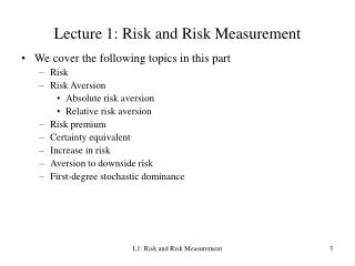
2. Transformations of Arrow-Pratt • Interpretations and Transformations of Scale for the Pratt-Arrow Absolute Risk Aversion coefficient: Implications for Generalized Stochastic Dominance • To this point, we have discussed technical manifestations of risk aversion such as where the risk aversion coefficient comes from and how the utility of income is derived. However, I want to start turning to the question: How do we apply the concept of risk aversion?

3. Several procedures exist for integrating risk into the decision making process such as direct application of expected utility, mathematical programming using the expected value-variance approximation, or the use of stochastic dominance. All of these approaches, however, require some notion of the relative size of risk aversion. • Risk aversion directly uses a risk aversion coefficient to parameterize the negative exponential or power utility functions.

4. Mathematical programming uses the concept of the tradeoff between variance and expected income. • Stochastic dominance uses measures of risk aversion to bound the utility function. • The current study gives some guidance on using previously published risk aversion coefficients. Specifically, the article looks at the effect of location and scale on the risk aversion coefficient • As a starting place, we develop an interpretation of the Pratt-Arrow coefficient in terms of marginal utility

6. This algebraic manipulation develops the absolute risk aversion coefficient as the percent change in marginal utility at any level of income. • Therefore, r is associated with a unit of change in outcome space. If the risk aversion coefficient was elicited in outcomes of dollars, then the risk aversion coefficient is .0001/$. • This result indicates that the decision-maker’s marginal utility is falling at a rate of .01% per dollar change in income.

7. This association between the risk aversion and the level of income then raises the question of the change in outcome scale. • For example, what if the original utility function was elicited on a per acre basis, and you want to use the results for a whole farm exercise? • Theorem 1: Let r(x)=u’’(x)/u’(x). Define a transformation of scale on x such that w=x/c, where c is a constant. Then r(w)=cr(x).

8. The proof lies in the change in variables. Given • In other words, if the scale of the outcome changes by c, the scale of the risk aversion coefficient must be changed by the same amount.

9. In other words, if the scale of the outcome changes by c, the scale of the risk aversion coefficient must be changed by the same amount. • Theorem 2: If v=x + c, where c is a constant, then r(v)=r(x). Therefore, the magnitude of the risk aversion coefficient is unaffected by the use of incremental rather absolute returns. • Example: Suppose that a study of U.S. farmers gives a risk aversion coefficient of r=.0001/$ (U.S.) Application to the Australian farmers whose dollar is worth .667 of the U.S. dollar is r=.0000667/$ Australian.

10. Mean-Variance Versus Direct Utility Maximization • Due to various financial economic models such as the Capital Asset Pricing Model that we will discuss in our discussion of market models, the finance literature relies on the use of mean-variance decision rules rather than direct utility maximization. • There is a practical aspect for stock-brokers who may want to give clients alternatives between efficient portfolios rather than attempting to directly elicit each individual’s utility function.

11. Along the later tack, the study by Kroll, Levy, and Markowitz examines the acceptability of the Mean-Variance procedure. Specifically, they attempt to determine whether the expected utility maximizing choice is contained in the Mean-Variance efficient set.

12. Two approaches for selecting the optimal portfolio of stock are to choose between the set of investments to maximize expected utility:

13. The second alternative is to map out the efficient Mean-Variance space by solving

14. A better formulation of the problem is And, where r is the Arrow Pratt absolute risk aversion coefficient

17. Meyer’s Location-Scale • Definition: Two cummulative distributions functions G1(.) and G2(.) are said to differ only by location and scale parameters and if G1(x) = G2( a+ b x) with > 0. • Several two-parameter families satisfy this property such as the normal and the uniform distributions.

18. Assume that there exists various choice sets, Yi, that only differ by location and scale parameters. • Let X be the random variable of one of these alternatives derived by normalizing by the mean and the standard deviation of the alternative

19. The expected utility of this alternative can then be derived as

20. The first step in examining the properties of V(s,m) is to examine its partial derivatives

21. Property 1: Vm(s,m) > 0 for all m and all s> 0 if and only if u’(a+bx) 0 for all a+bx. • Property 2: Vs(s,m) < 0 for all m and all s> 0 if and only if u’’(a+bx) 0 for all a+bx.. • Property 1 states that increases in increase V(.) if the marginal utility u’(.) is positive. Similarly, increases in reduce V(.) if the utility function is concave. Defining S(,) as

23. Property 3: S(s,m) >= 0 for all m and all s>0 if and only if u’(a+bx) >0 and u’’(a+bx) <0 for all a+bx.

24. Property 4: V(s,m) is a concave function for all m and all s>0 if and only if u’’(a+bx) 0 for all a+bx. • Property 5: dS(s,m)/ dm < (=,>) 0 for m and all s > 0 if and only if u(a+bx) displays decreasing (constant, increasing) absolute risk aversion for all a+bx.

25. Property 6: d S(ts,tm)/ dt < (=,>) 0 for m and all s> 0 if and only if u(a+bx) displays decreasing (constant, increasing) absolute risk aversion for all a+bx. • Property 7: S1(s,m) >= S2(s,m) for all (s,m) if and only if u1(a+bx) is more risk averse than u2(a+bx).