Download
1 / 55
650 likes | 768 Views
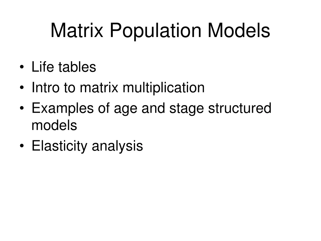
Matrix Population Models. Life tables Intro to matrix multiplication Examples of age and stage structured models Elasticity analysis. Life Tables and Matrices: Accounting demographic parameters. Killer Whale Lefkovich matrix from Brault, S. and H. Caswell (1993).

E N D
Matrix Population Models • Life tables • Intro to matrix multiplication • Examples of age and stage structured models • Elasticity analysis
Life Tables and Matrices:Accounting demographic parameters Killer Whale Lefkovich matrix from Brault, S. and H. Caswell (1993) Sardine life table(Sardinops sagax) from Murphy (1967)
Matrix multiplication Scalar Multiplication - each element in a matrix is multiplied by a constant.
Matrix multiplication Multiply rows times columns. You can only multiply if the number of columns in the 1st matrix is equal to the number of rows in the 2nd matrix.
Matrix multiplication Multiply rows times columns. You can only multiply if the number of columns in the 1st matrix is equal to the number of rows in the 2nd matrix. Dimensions: 3 x 2 2 x 3 They must match. The dimensions of your answer.
2 x 2 2 x 2 *Answer should be dimension ? 0(4) + (-1)(-2) 0(-3) + (-1)(5) 1(4) + 0(-2) 1(-3) +0(5)
Matrix Multiplication (Population Model): x = Answer should be dimension ?
Introduction to Matrix Models • Vital rates describe the development of individuals through their life cycle (Caswell 1989) • Vital rates are : birth, growth, development, reproductive, mortality rates • The response of these rates to the environment determines: • population dynamics in ecological time • the evolution of life histories in evolutionary time
The general form of an age-structured Leslie Matrix models “Projection Matrix”:
The general form of an age-structured Leslie Matrix models “Projection Matrix”:
Age Class 4 Age based matrix population model • Fecundity fx • Survivorship sx Age Class 3 Age Class 1 Age Class 2
The general form of Lefkovitch Matrix modelStage – structured Projection Matrix
The general form of Lefkovitch Matrix modelStage – structured Projection Matrix
Size Class 4 Stage-based matrix population model • Fecundity fx • Growth gx and Survivorship sx Size Class 3 Size Class 1 Size Class 2
Some of the utility of matrix population models • Population projection – deterministic and stochastic • Elasticity Analysis • Conservation • Management • Meta population dynamics
Caswell • Types of model variability
Population projectionExample: What is the population at t1? Juvenile Adult t0 fx NJuvenile NAdult px
x = fx Juvenile Adult px
Projecting this sample matrix indefinitely will result in the finite population growth rate: λ t0 x =
Look at the y-axis λ is on the natural log scale…
Elasticity: Proportional sensitivity (of λ ) to matrix element perturbations λ = 2.00 A 25% decrease in Age 1 survivorship results in a 12% decrease in population growth. λ = 1.76
Elasticity: Proportional sensitivity (of λ ) to matrix element perturbations λ = 2.00 A 25% increase in Age 2 fecundity results in a 9% increase in population growth. λ = 2.18
Elasticity • A type of “perturbation” analysis • The elasticityeijindicates the relative impact on of a modification of the value of the parameteraij • Scaled, therefore The elasticityisindependent on the metric of the parameteraij and
Stage-specific survival and reproduction • G, P, F
Stage-specific survival and reproduction • G, P, F
Stage-specific survival and reproduction • Initialize matrix A
‘A size-based projection matrix model and elasticity analysis of red abalone, Haliotis rufescens, in northern California.’ Robert Leaf and Laura Rogers-Bennettrleaf@mlml.calstate.edu Moss Landing Marine Laboratories U.C. Bodega Marine Laboratory This work was funded by SeaGrant Traineeship # R/CZ-69PD TR
Abalone harvest in California Adapted from Karpov et al. 2000
North of San Francisco Bay Only red abalone may be taken 7 inch limit (178 mm) Free-dive only (no SCUBA) 3 red abalone per day Maximum take: 24 abalone during a calendar year Recreational abalone fishery
What are the most effective conservation measures for red abalone? • “Outplanting” or seeding juveniles • Increase juvenile survivorship • Marine Protected Areas • Increase adult survivorship (>178 mm) and eliminate incidental mortality • New Size Limits • Are current limits set appropriately?
Size Class 4 Size based matrix population model • Fecundity fx • Growth gx • Survivorship sx Size Class 3 Size Class 1 Size Class 2
ElasticityExample if ei,j = 0.510% change in the value of a parameter (ai,j) will result in a 5% increase in the population growth rate.
Annual growthCDFG Tagging study 1971 – 1978 (Schultz and DeMartini unpublished) • Red abalone tagged at the five sites (n = 5997) • 41.5 to 222 mm SL • 845 recaptured at one year intervals plus or minus 30 days (335 to 395 days) • Growth was normalized to one year. Mendocino county Pt. Cabrillo (N. and S.) Van Damme SP Pt. Arena Sonoma county Ft. Ross
Growth transition matrix - gx Size class (mm) t0 Size class (mm)t1 Number of indivuals in size class at t0
Growth transition frequencies - gx Size class (mm) t0 Size class (mm)t1
Size Class 4 Size based matrix population model • Fecundity fx • Growth gx • Survivorship sx Size Class 3 Size Class 1 Size Class 2
Annual Survival Estimates Individual tag number Julian Day Annual Model Name Number of individuals Survival Estimate Standard Error ‘cryptic’ (< 100 mm) 179 0.525 0.0506 ‘emergent’ (≥ 100 mm) 567 0.691 0.0240
Incorporation of annual survivalrates into growth transition frequencies x 0.525 y -1 x 0.691 y -1
Incorporation of annual survivalrates into growth transition frequencies
Size Class 4 Size based matrix population model • Fecundity fx • Growth gx • Survivorship sx Size Class 3 Size Class 1 Size Class 2
Incorporate fecundities (number of eggs) and solve for first year survivorship assuming a stable population growth rate. 113 * 105 x P0 So, P0 = 1.5 x 10⁻⁶, approximately 1 individual in 665,000 survives to the beginning of their second year
Elasticity results Current size limit 178 mm
What are the most effective conservation measures for red abalone? • “Outplanting” or seeding juveniles • Increase juvenile survivorship • Marine Protected Areas • Increase adult survivorship (>178 mm) and eliminate incidental mortality • New Size Limits • Are current limits set appropriately?
Elasticity results Current size limit 178 mm