Download
1 / 65
650 likes | 664 Views
Turbulent Origins of the Sun’s Hot Corona and the Solar Wind. Steven R. Cranmer Harvard-Smithsonian Center for Astrophysics. Turbulent Origins of the Sun’s Hot Corona and the Solar Wind. Outline: Solar overview: Our complex “variable star” How do we measure waves & turbulence?

E N D
Turbulent Origins of the Sun’s Hot Corona andthe Solar Wind Steven R. CranmerHarvard-SmithsonianCenter for Astrophysics
Turbulent Origins of the Sun’s Hot Corona andthe Solar Wind • Outline: • Solar overview: Our complex “variable star” • How do we measure waves & turbulence? • Coronal heating & solar wind acceleration • Preferential energization of heavy ions Steven R. CranmerHarvard-SmithsonianCenter for Astrophysics
Motivations for “heliophysics” • Space weather can affect satellites, power grids, and astronaut safety. • The Sun’s mass-loss & X-ray history impacted planetary formation and atmospheric erosion. • The Sun is a unique testbed for many basic processes in physics, at regimes (T, ρ, P) inaccessible on Earth . . . • plasma physics • nuclear physics • non-equilibrium thermodynamics • electromagnetic theory
The Sun’s overall structure • Core: • Nuclear reactions fuse hydrogen atoms into helium. • Radiation Zone: • Photons bounce around in the dense plasma, taking millions of years to escape the Sun. • Convection Zone: • Energy is transported by boiling, convective motions. • Photosphere: • Photons stop bouncing, and start escaping freely. • Corona: • Outer atmosphere where gas is heated from ~5800K to several million degrees!
The extended solar atmosphere The “coronal heating problem”
The solar photosphere • In visible light, we see top of the convective zone (wide range of time/space scales): β << 1 β ~ 1 β > 1
The solar chromosphere • After T drops to ~4000 K, it rises again to ~20,000 K over 0.002 Rsun of height. • Observations of this region show shocks, thin “spicules,” and an apparently larger-scale set of convective cells (“super-granulation”). • Most… but not all… material ejected in spicules appears to fall back down. (Controversial?)
The solar corona • Plasma at 106 K emits most of its spectrum in the UV and X-ray . . . Coronal hole (open) “Quiet” regions Active regions
The coronal heating problem • We still do not understand the physical processes responsible for heating up the coronal plasma. A lot of the heating occurs in a narrow “shell.” • Most suggested ideas involve 3 general steps: 1. Churning convective motions that tangle up magnetic fields on the surface. 2. Energy is stored in twisted/braided/swaying magnetic flux tubes. 3.Something releases this energy as heat. Particle-particle collisions? Wave-particle interactions? “I think you should be more explicit here in step two.”
A small fraction of magnetic flux is OPEN Peter (2001) Fisk (2005) Tu et al. (2005)
2008 Eclipse: M. Druckmüller (photo) S. Cranmer (processing) Rušin et al. 2010 (model)
In situ solar wind: properties • 1958: Eugene Parker proposed that the hot corona provides enough gas pressure to counteract gravity and produce steady supersonic outflow. • Mariner 2 (1962): first confirmation of fast & slow wind. • 1990s: Ulysses left the ecliptic; provided first 3D view of the wind’s source regions. • 1970s: Helios (0.3–1 AU). 2007: Voyagers @ term. shock! fast slow 300–500 high chaotic all ~equal more low-FIP speed (km/s) density variability temperatures abundances 600–800 low smooth + waves Tion >> Tp > Te photospheric
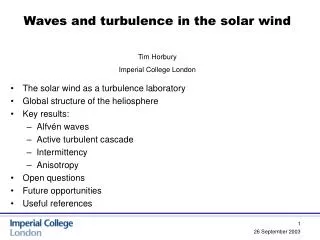
Outline: • Solar overview: Our complex “variable star” • How do we measure solar waves & turbulence? • Coronal heating & solar wind acceleration • Preferential energization of heavy ions
Waves & turbulence in the photosphere • Helioseismology: direct probe of wave oscillations below the photosphere (via modulations in intensity & Doppler velocity) • How much of that wave energy “leaks” up into the corona & solar wind? Still a topic of vigorous debate! • Measuring horizontal motions of magnetic flux tubes is more difficult . . . but may be more important? splitting/merging torsion 0.1″ longitudinal flow/wave bending (kink-mode wave)
Waves in the corona • Remote sensing provides several direct (and indirect) detection techniques: • Intensity modulations . . . • Motion tracking in images . . . • Doppler shifts . . . • Doppler broadening . . . • Radio sounding . . . SOHO/LASCO (Stenborg & Cobelli 2003)
Wavelike motions in the corona • Remote sensing provides several direct (and indirect) detection techniques: • Intensity modulations . . . • Motion tracking in images . . . • Doppler shifts . . . • Doppler broadening . . . • Radio sounding . . . Tomczyk et al. (2007)
In situ fluctuations & turbulence • Fourier transform of B(t), v(t), etc., into frequency: f -1 energy containing range f -5/3 inertial range The inertial range is a “pipeline” for transporting magnetic energy from the large scales to the small scales, where dissipation can occur. Magnetic Power f -3dissipation range few hours 0.5 Hz
Alfvén waves: from photosphere to heliosphere • Cranmer & van Ballegooijen (2005) assembled much of the existing data togethter: Hinode/SOT SUMER/SOHO G-band bright points UVCS/SOHO Helios & Ulysses Undamped (WKB) waves Damped (non-WKB) waves
Outline: • Solar overview: Our complex “variable star” • How do we measure solar waves & turbulence? • Coronal heating & solar wind acceleration • Preferential energization of heavy ions
What processes drive solar wind acceleration? Two broad paradigms have emerged . . . • Wave/Turbulence-Driven (WTD) models, in which flux tubes stay open. • Reconnection/Loop-Opening (RLO) models, in which mass/energy is injected from closed-field regions. vs. • There’s a natural appeal to the RLO idea, since only a small fraction of the Sun’s magnetic flux is open. Open flux tubes are always near closed loops! • The “magnetic carpet” is continuously churning (Cranmer & van Ballegooijen 2010). • Open-field regions show frequent coronal jets (SOHO, STEREO, Hinode, SDO).
Waves & turbulence in open flux tubes • Photospheric flux tubes are shaken by an observed spectrum of horizontal motions. • Alfvén waves propagate along the field, and partly reflect back down (non-WKB). • Nonlinear couplings allow a (mainly perpendicular) cascade, terminated by damping. (Heinemann & Olbert 1980; Hollweg 1981, 1986; Velli 1993; Matthaeus et al. 1999; Dmitruk et al. 2001, 2002; Cranmer & van Ballegooijen 2003, 2005; Verdini et al. 2005; Oughton et al. 2006; many others)
Turbulent dissipation = coronal heating? • In hydrodynamics, von Kármán, Howarth, & Kolmogorov worked out cascade energy flux via dimensional analysis: • In MHD, cascade is possible only if there are counter-propagating Alfvén waves… (“cascade efficiency”) Z– Z+ • n = 1: an approximate “golden rule” from theory • Caution: this is an order-of-magnitude scaling. (e.g., Pouquet et al. 1976; Dobrowolny et al. 1980; Zhou & Matthaeus 1990; Hossain et al. 1995; Dmitruk et al. 2002; Oughton et al. 2006) Z–
Implementing the wave/turbulence idea • Cranmer et al. (2007) computed self-consistent solutions for waves & background plasma along flux tubes going from the photosphere to the heliosphere. • Only free parameters: radial magnetic field & photospheric wave properties. (No arbitrary “coronal heating functions” were used.) • Self-consistent coronal heating comes from gradual Alfvén wave reflection & turbulent dissipation. • Is Parker’s critical point above or below where most of the heating occurs? • Models match most observed trends of plasma parameters vs. wind speed at 1 AU. Ulysses 1994-1995
Cranmer et al. (2007): other results Wang & Sheeley (1990) ACE/SWEPAM ACE/SWEPAM Ulysses SWICS Ulysses SWICS Helios (0.3-0.5 AU)
Understanding physics reaps practical benefits 3D global MHD models Real-time space weather predictions? Self-consistent WTD models Z– Z+ Z–
Outline: • Solar overview: Our complex “variable star” • How do we measure solar waves & turbulence? • Coronal heating & solar wind acceleration • Preferential energization of heavy ions
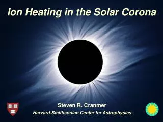
Coronal heating: multi-fluid, collisionless UVCS/SOHO O+5 O+6 p+ e– In the lowest density solar wind streams . . . electron temperatures proton temperatures heavy ion temperatures
Alfven wave’s oscillating E and B fields ion’s Larmor motion around radial B-field Preferential ion heating & acceleration • Parallel-propagating ion cyclotron waves (10–10,000 Hz in the corona) have been suggested as a natural energy source . . . instabilities dissipation lower qi/mi faster diffusion (e.g., Cranmer 2001)
However . . . Does a turbulent cascade of Alfvén waves (in the low-beta corona) actually produce ion cyclotron waves? Most models say NO!
Anisotropic MHD turbulence • When magnetic field is strong, the basic building block of turbulence isn’t an “eddy,” but an Alfvén wave packet. k ? Energy input k
Anisotropic MHD turbulence • When magnetic field is strong, the basic building block of turbulence isn’t an “eddy,” but an Alfvén wave packet. • Alfvén waves propagate ~freely in the parallel direction (and don’t interact easily with one another), but field lines can “shuffle” in the perpendicular direction. • Thus, when the background field is strong, cascade proceeds mainly in the plane perpendicular to field (Strauss 1976; Montgomery 1982). k Energy input k
Anisotropic MHD turbulence • When magnetic field is strong, the basic building block of turbulence isn’t an “eddy,” but an Alfvén wave packet. • Alfvén waves propagate ~freely in the parallel direction (and don’t interact easily with one another), but field lines can “shuffle” in the perpendicular direction. • Thus, when the background field is strong, cascade proceeds mainly in the plane perpendicular to field (Strauss 1976; Montgomery 1982). k ion cyclotron waves Ωp/VA kinetic Alfvén waves • In a low-β plasma, cyclotron waves heat ions & protons when they damp, but kinetic Alfvén waves are Landau-damped, heating electrons. Energy input k Ωp/cs
Parameters in the solar wind • What wavenumber angles are “filled” by anisotropic Alfvén-wave turbulence in the solar wind? (gray) • What is the angle that separates ion/proton heating from electron heating? (purple curve) θ k k Goldreich &Sridhar (1995) electron heating proton & ion heating
Nonlinear mode coupling? • There is observational evidence for compressive (non-Alfvén) waves, too . . . (e.g., Krishna Prasad et al. 2011) Can Alfvén waves (left-hand polarized) couple with fast-mode waves (right-hand polarized)?
Preliminary coupling results • Chandran (2005) suggested that weak turbulence couplings (AAF, AFF) may be sufficient to transfer enough energy to Alfvén waves at high parallel wavenumber. • New simulations in the presence of strong Alfvénic turbulence (e.g., Goldreich & Sridhar 1995) show that these couplings may give rise to wave power that looks like a kind of “parallel cascade” (Cranmer, Chandran, & van Ballegooijen 2011) r = 2 Rs β ≈ 0.003
Other ideas . . . • When MHD turbulence cascades to small perpendicular scales, the small-scale shearing motions may be unstable to the generation of ion cyclotron waves (Markovskii et al. 2006). • Turbulence may lead to dissipation-scale current sheets that may preferentially spin up ions (Dmitruk et al. 2004). • If there are suprathermal tails in chromospheric velocity distributions, then collisionless velocity filtration (Scudder 1992) may give heavy ions much higher temperatures than protons (Pierrard & Lamy 2003). • If nanoflare-like reconnection events in the low corona are frequent enough, they may fill the extended corona with electron beams that would become unstable and produce ion cyclotron waves (Markovskii 2007). • If kinetic Alfvén waves reach large enough amplitudes, they can damp via stochastic wave-particle interactions and heat ions (Voitenko & Goossens 2006; Wu & Yang 2007; Chandran 2010). • Kinetic Alfvén wave damping in the extended corona could lead to electron beams, Langmuir turbulence, and Debye-scale electron phase space holes which could heat ions perpendicularly (Matthaeus et al. 2003; Cranmer & van Ballegooijen 2003).
Conclusions • Advances in MHD turbulence theory continue to help improve our understanding about coronal heating and solar wind acceleration. • It is becoming easier to include “real physics” in 1D → 2D → 3D models of the complex Sun-heliosphere system. • However, we still do not have complete enough observational constraintsto be able to choose between competing theories. SDO/AIA For more information: http://www.cfa.harvard.edu/~scranmer/
The outermost solar atmosphere • Total eclipses let us see the vibrant outer solar corona: but what is it? • 1870s: spectrographs pointed at corona: • 1930s: Lines identified as highly ionized ions: Ca+12 , Fe+9 to Fe+13 it’s hot! • Fraunhofer lines (not moon-related) • unknown bright lines • 1860–1950: Evidence slowly builds for outflowing magnetized plasma in the solar system: • solar flares aurora, telegraph snafus, geomagnetic “storms” • comet ion tails point anti-sunward (no matter comet’s motion) • 1958: Eugene Parker proposed that the hot corona provides enough gas pressure to counteract gravity and accelerate a “solar wind.”
Wave / Turbulence-Driven models • Cranmer & van Ballegooijen (2005) solved the transport equations for a grid of “monochromatic” periods (3 sec to 3 days), then renormalized using photospheric power spectrum. • One free parameter: base “jump amplitude” (0 to 5 km/s allowed; ~3 km/s is best)
Self-consistent 1D models • Cranmer, van Ballegooijen, & Edgar (2007) computed solutions for the waves & background one-fluid plasma state along various flux tubes... going from the photosphere to the heliosphere. • The only free parameters: radial magnetic field & photospheric wave properties. • Some details about the ingredients: • Alfvén waves: non-WKB reflection with full spectrum, turbulent damping, wave-pressure acceleration • Acoustic waves: shock steepening, TdS & conductive damping, full spectrum, wave-pressure acceleration • Radiative losses: transition from optically thick (LTE) to optically thin (CHIANTI + PANDORA) • Heat conduction: transition from collisional (electron & neutral H) to a collisionless “streaming” approximation
Magnetic flux tubes & expansion factors A(r) ~ B(r)–1 ~ r2 f(r) (Banaszkiewicz et al. 1998) Wang & Sheeley (1990) defined the expansion factor between “coronal base” and the source-surface radius ~2.5 Rs. TR polar coronal holes f ≈ 4 quiescent equ. streamers f ≈ 9 “active regions” f ≈ 25
Results: turbulent heating & acceleration T (K) Ulysses SWOOPS Goldstein et al. (1996) reflection coefficient
Results: flux tubes & critical points • Wind speed is ~anticorrelated with flux-tube expansion & height of critical point. Cascade efficiency: n=1 n=2 rcrit rmax (where T=Tmax)
Results: heavy ion properties • Frozen-in charge states • FIP effect (using Laming’s 2004 theory) Ulysses SWICS Cranmer et al. (2007)
Results: in situ turbulence • To compare modeled wave amplitudes with in-situ fluctuations, knowledge about the spectrum is needed . . . • “e+”: (in km2 s–2 Hz–1 ) defined as the Z– energy density at 0.4 AU, between 10–4 and 2 x 10⁻⁴ Hz, using measured spectra to compute fraction in this band. Helios (0.3–0.5 AU) Tu et al. (1992) Cranmer et al. (2007)
B ≈ 1500 G (universal?) f ≈ 0.002–0.1 B ≈ f B , . . . . . . • Thus, . . . and since Q/Q ≈ B/B , the turbulent heating in the low corona scales directly with the mean magnetic flux density there (e.g., Pevtsov et al. 2003; Schwadron et al. 2006; Kojima et al. 2007; Schwadron & McComas 2008). Results: scaling with magnetic flux density • Mean field strength in low corona: • If the regions below the merging height can be treated with approximations from “thin flux tube theory,” then: B ~ ρ1/2 Z± ~ ρ–1/4 L┴ ~ B–1/2
Mirror motions select height • UVCS “rolls” independently of spacecraft • 2 UV channels: • 1 white-light polarimetry channel LYA (120–135 nm) OVI (95–120 nm + 2nd ord.) The UVCS instrument on SOHO • 1979–1995: Rocket flights and Shuttle-deployed Spartan 201 laid groundwork. • 1996–present: The Ultraviolet Coronagraph Spectrometer (UVCS) measures plasma properties of coronal protons, ions, and electrons between 1.5 and 10 solar radii. • Combines “occultation” with spectroscopy to reveal the solar wind acceleration region! slit field of view: