Douglas R. W hite , Bahattin Tolga Oztan , John Snarey

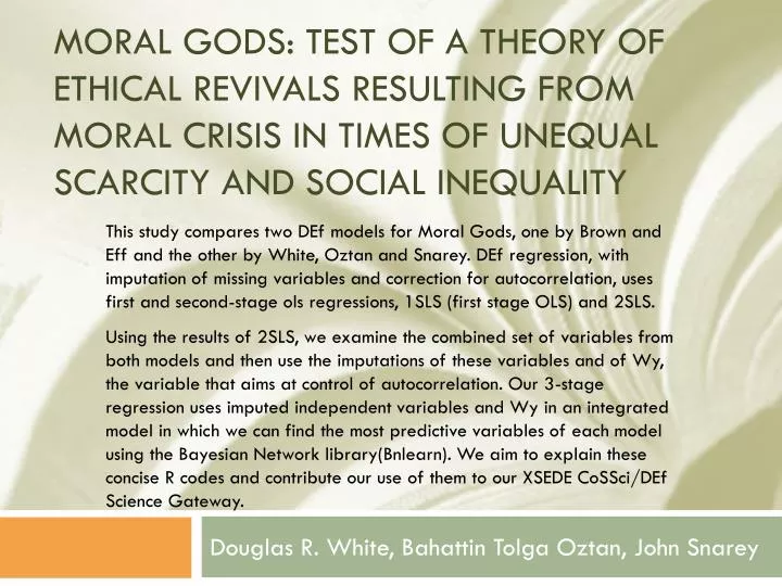
1. This study compares two DEf models for Moral Gods, one by Brown and Eff and the other by White, Oztan and Snarey. DEf regression, with imputation of missing variables and correction for autocorrelation, uses first and second-stage ols regressions, 1SLS (first stage OLS) and 2SLS. Using the results of 2SLS, we examine the combined set of variables from both models and then use the imputations of these variables and of Wy, the variable that aims at control of autocorrelation. Our 3-stage regression uses imputed independent variables and Wy in an integrated model in which we can find the most predictive variables of each model using the Bayesian Network library(Bnlearn). We aim to explain these concise R codes and contribute our use of them to our XSEDE CoSSci/DEf Science Gateway. Moral gods: TEST OF A THEORY of ETHICAL REVIVALS Resulting from MORAL CRISIS in times of unequal scarcity and social inequality Douglas R. White, Bahattin Tolga Oztan, John Snarey

2. Outline of Slides ABQhiGodPresentation2014.pptx *p3-4 Theory: Crises of inequality in polities with exchange systems Many such examples studied by Peter Turchin (2005 etc) *5 Example: Han dynasty collapse & Moral crisis *6 Defining KeyTheoretical Variables (FxCmntyWages, AnimXbwealth, SuperjhWriting) *7 Wy term regression: Model equations used in comparison Brown&Eff 2010 White et al *8 Wy 2SLS term regression results *9 CoSSci/DEf 2SLS modelingresults for HiGods: Key theoretical & other variables *10 3stage regression results with imputed variables: White et al. (2011) Brown & Eff (2010) *11 3-stage modelusesimputed variables & est(Wy) & allows Bayesian Network Learning *12 Bayesian Network Graph and Cross-tabs *13 Trestles bootstraps, alternative models, Paul Rodriguez *14 Paul Rodriguez use of library(bootstrap) to show alternate Bayesian Networks *15 Questions about Bayesian Networks (belongs after p.13 in longer talk) *16 Summary: Null Hypotheses and Comparison of Results model: Ev2007Higod4.xls Trailing Questions Do our results differ drastically from the usual OLS regression? Yes Recap of 3-stage Regression with imputed variables that includes the estimated Wy and results What is Bayesian Network Learning, a Bayesian Network, and library(bnlearn)? False hopes; Bivariate distributions; Recap of Def 2SLS and 3-stage regression

3. Han China shows one of many examples of exchange system political dynamics that create MORAL CRISIS periods. Two full cycles over 500 years are shown in the Phase diagram to the right and in cycles below (phase diagram is actually from another example) Turchin 2005: Dynamical Feedbacks in Structural Demography Rise +Pop-conf Peace -Pop-conf Conflict +Pop+cnf Crash -P+conf Key: =Innovation phases Inequality & crashes p.3 Chinese phase diagram

4. p.4

5. Example: Han dynasty collapse & Moral crisis followed by adoption of Buddhism p.5 Confucianism originated as an "ethical-sociopolitical teaching" during the Spring and Autumn Period, but later developed metaphysical and cosmological elements in the Han Dynasty. Following the official abandonment of Legalism in China after the Qin Dynasty, Confucianism became the official state ideology of the Han. Nonetheless, from the Han period onward, most Chinese emperors have used a mix of Legalism and Confucianism as their ruling doctrine, often with the latter embellishing the former. In other words, Confucian values were used to sugar-coat the harsh Legalist ideas that underlie the Imperial system. The disintegration of the Han in the second century CE opened the way for the spiritual and otherworldly doctrines of Buddhism and Daoism to dominate intellectual life at that time.” Wikipedia: Confucianism.

6. Defining key theoretical variables p. 6 *FxCmtyWages= Wages x Fixed community ((v2125>1)*1)*(v61==6)*1 concept: Given wages in communities where land is owned, inequality is amplified in extended periods of resource scarcity. When due to overpopulation, the value of property increases relative to oversupply of workers whose wages are lowered, a potential context for extreme inequality. *AnimXbwealth = (% Pastoralism v206) x (Bridewealth v208=1) concept: (a) owner lineages of herds of camels and horses employ suborned lineages as herders and caravan workers. (b) In times of extreme scarcity following population increase that outruns food supply, plentiful workers are of lesser value (c) herd ownership is of excess value due to scarcity, and (d) if brideprice is present, owners have a more extreme advantages in acquiring multiple wives from lesser lineages. *SuperjhWriting= Superjurisdictiocal Hierarchy x Writing v237*(1+((v149>=3)*1)) concept: In such Malthusian crises as above, taxes relative to income pose a potential context for extreme inequality.

7. Wy term Regression: comparing models of White,Oztan,Snarey and Brown and Eff p.7 W is a weighted sum of square zero-diagonal matrices (inverse distance, language similarities) with row sums normalized to 1, so that the product Wy measures interdependencies in the dependent variable y and is thus suitable as a control for autocorrelation in a regression equation for the dependent variable y. An initial regression (1sls) estimates the Wy dependent variable using the columns of WXas predictor variables, i.e., estimate Wy = a + WXc + υand save the vector of estimated scores ŷw = â + WXĉ, whereŷwis now a suitable control variable for autocorrelation of the dependent variable y. DEf first imputes all variables, then estimates ŷw. Then, a second ols regression (2), the 2SLSDow-Eff equation (DEf), estimates the βiXicoefficientsβiand the autocorrelation coefficient ρ (of ŷw ) that together predict the dependent variable y.

8. Ŷw term 2SLS RegressionResults p. 8 (2) y = β0 +ρŷw +β1X1 + β2X2 +…+ βKX2K + ε e.g. testing HiGod predictors of White etal and Brown & Eff Slide 9 shows results of 2SLS regression for significant variables at p < .10: six are those of White et al(AnimXbwealth, No_Rain_Dry, Writing, Missions, bio.5, and Distant Father, plus PCsizeSq– also significant in Brown & Eff), and Caste is a second significant Brown & Eff variable. FxCmtyWages, at p < 0.14 as a predictor in this model, is not significant. 3-stage Regression Results Slide 10shows how imputed rather than raw variables, used in a third ols regression, elevates the FxCmtyWages variable to significance, as proposed from prior theory.

9. DEf 2SLS results for HiGods p. 9

10. 3-stage regression with imputed variables: White et al (bold or red) vs. Brown & Eff p.10 Coefficients: Estimate Std. Error t value Pr(>|t|) (Intercept) 0.006272 0.473491 0.013 0.98945 Wy 0.651359 0.136649 4.767 0.00061 *** FxCmtyWages* 0.751684 0.259420 2.898 0.00426 ** Missions 0.334426 0.140836 2.375 0.01868 * bio.5 (temp) -0.150861 0.079799 -1.891 0.06039 . PCsizeSq** -0.077855 0.041264 -1.887 0.06090 . Writing 0.115742 0.064661 1.790 0.07524 . Caste 0.171590 0.104619 1.640 0.10283 AnimXbwealth 0.090378 0.059296 1.524 0.12932 DistantFather -0.129960 0.087188 -1.491 0.13793 No_rain_Dry 0.120057 0.083832 1.432 0.15395 PCsize 0.102367 0.078573 1.303 0.19440 ExtWar -0.013503 0.010783 -1.252 0.21221 AgPot -0.053785 0.064506 -0.834 0.40556 FoodScarcity 0.018975 0.056114 0.338 0.73567 Anim -0.006878 0.057393 -0.120 0.90476 *The FxCmtyWages variable is, as hypothesized, significant. **Works in both models. All variables imputed for n=186

11. The 3-stage model uses regression-imputed variables Xh and ŷw & facilitates Bayesian Network Learning p.11 (3) y = β0 +ρŷw +β1Xh1+β2Xh2 +…+ βKXh2K + ε A new regression model uses the imputed variables Xh: HiGod <- h$data[,"HiGod"] h$data[, retrieves imputed vars AnimXbwealth <- h$data[,"AnimXbwealth"] No_rain_Dry <- h$data[,"No_rain_Dry"] Writing <- h$data[,"v149"] AgPot <- h$data[,"PCAP"] PCsizeSq <- h$data[,"PCsizeSq"], etc. The function h$data[…] denotes imputed variables whether data are missing or not. A 4th-stage analysis compares the White et al and Brown and Eff models byjoint analysis of all of their 3-stage variables and allows the use of Bayesian Network Learningwith R library(bnlearn), newly available in 2014.

12. Bayesian Network Learning Results using imputed data and library(bnlearn) in comparing the two Moral Gods models p.12 Bayesian Network Learning Results p.13 AnimXbwealth HiGod0 1 2 3 4 5 7 8 9 1 54 7 6 1 0 0 0 1 0 2 40 6 5 0 0 0 0 0 0 3 13 1 4 3 1 0 1 0 0 4 21 2 0 9 3 1 0 3 4 White, Oztan & Snarey (2014) Brown & Eff (2010) HiGod FxCmtyWages 1 2 3 4 0 43 27 11 17 1 18 11 5 23 3=neither Islam nor Christianity 4=supportive of morality Writing & Records HiGod1 2 3 4 5 1 35 16 10 0 8 2 25 17 6 0 3 3 7 9 3 2 2 4 6 7 2 10 18

13. Trestles bootstraps, Paul Rodriguez p.13 Next, a bootstrap procedure was used to explore the distribution of possible network models (Efron & Tishbrini, 1986). One thousand bootstrap resamples were taken by sampling the original dataset with replacement. For each new sample dataset, a bayes network was found using the grow-shrink algorithm (heeding independencies in the data). The binary valued adjacency matrix for each network was saved and then averaged across all 1000 networks, thereby producing an expectation for the presence of every edge (Figure with graph in file named 'BNwboot_nowy_05thresh'). This approach has proved very useful in biological network discovery (e.g. Marbach, etal. 2012). The expectation serves as a weight on the edge, but it does not indicate what typical networks appear in the bootstrap samples. Therefore, we also sorted and counted the adjacency matrices, and printed out the most frequent networks. Efron, B.; Tibshirani, R. 1993. An Introduction to the Bootstrap. Chapman & Hall/CRC. Marbach D, Costello JC, Küffner R, Vega NM, Prill RJ, Camacho DM, Allison KR; The DREAM5 Consortium, Kellis M, Collins JJ, Stolovitzky G. 2012. Wisdom of crowds for robust gene network inference. Nature Methods9(8):796-804. 58 collaborators.Margaritis, D. and Thrun, S. 2000. Bayesian network induction via local neighborhoods. In Advances in Neural Information Processing Systems 12. (“the bootstrap.”)

14. library(bootstrap) blocLite(Rgraphviz)

15. Bioconductor.blocLite.R library(bootstrap) Paul Rodriguez SDSCblocLite(Rgraphviz)V=letters[1:10]M=1:4g1=randomGraph(V,M,0.2)plot(g1)Probabilities are generated by bootstrap, run on SDSC Trestles supercomputer 1695=No Scarification, 270=Class stratificationp. 13b (shown in session discussion #2)

16. Questions about Bayesian Networks p.14 • *Why are ab identifiable? Because there is no observed variable or bias that significantly affect them both (KF:1024). • Does subtraction of variables alter a BN graph?No. Addition? • Only if the above* is violated (strengthened by many candidates). • If you add x and get axb will that change a BN?No. Since .. are probabilities, their product is a probability but a to b may have other additive probabilities from other paths. axb? Yes. • Does subsampling cases in the same time period alter a BN? Yes. W matrices and PCs for imputing data are subsampled too. • Why do significances change between DEf and Wy Reg? Entry of est(Wy) is an additional variable... KF=Koller & Friedman 2009. Probabilistic Graphical Models.

17. SUMMARY: Null Hypotheses and Comparison of Results p.15 The null hypothesis for the pvalues in our models is that the true value of the coefficient is zero. For Moral Gods: The Autocorrelation regression model tells us that that some theoretically-derived variables are significant. The Wy term imputed variable regressionalso shows an especially significant effect of FxCmntyWages but for moral gods unconcerned with humans. The Wy term Bayesian Network shows potential causality of FxCmntyWages and AnimXbwealth. The Bootstrap shows probabilistic alternative models, several with indirect effects, each with the central theoretical variables, FxCmntyWages and AnimXbwealth.

18. Questions/Discussions OTHER QUESTIONS? Christian Brown and Anthon Eff. 2010. The State and the Supernatural: Support for Prosocial Behavior, Structure and Dynamics: eJournal of Anthropological Sciences 4(1). Douglas R. White, B. Tolga Oztan, Giorgio Gosti, Elliott Wagner, and John Snarey. 2010. Discovery of Hidden Variables for the Evolution of Ethical Religions. Submitted to Scientific American. Douglas R. White, B. Tolga Oztan, and John Snarey. 2014. Moral gods. ABQ session.

19. Question: In regard to autocorrelation, i.e., Galton’s problem, do our results differ from OLS? Yes, very much. • Estimate Std. Error t value Pr(>|t|) • (Intercept) 1.019415 0.729651 1.397 0.16577 • dx$FxCmtyWages 0.023184 0.273012 0.085 0.93251 • dx$v2006 Missions 0.457471 0.220324 2.076 0.04068 * • dx$v149 Writing 0.260651 0.104351 2.498 0.01429 * • dx$v272 0.193109 0.182208 1.060 0.29203 • dx$AnimXbwealth 0.105582 0.079593 1.327 0.18798 • dx$v3 -0.003290 0.072426 -0.045 0.96387 • dx$No_rain_Dry 0.340791 0.126310 2.698 0.00831 ** • dx$v1650 -0.012738 0.015911 -0.801 0.42546 • dx$v1685 -0.038787 0.082818 -0.468 0.64066 • dx$v206 -0.008370 0.072604 -0.115 0.90848 • dx$bio.5 -0.002922 0.001762 -1.659 0.10064 • PCAP 0.139448 0.101782 1.370 0.17404 • PCsize 0.025052 0.140601 0.178 0.85898 • PCsizeSq -0.054963 0.057641 -0.954 0.34284

20. Recap of 3-stage Regression with imputed variables that includes the estimated Wy and results • Once DEf is run, Wy is defined along with imputed variables. A simple OLS regression can be run where y = β0+β1Wy + βiimputed(Xi)+ ε • This model gives a total Rsq including Wy, and somewhat different coefficients and significances. ____FxCmtyWages is the most significant variable. AnimXbridewealth is close to significance and less significant than in DEf. Five variables are significant. All belong to the White et al., one shared with Brown and Eff (2010), one exclusive to Brown and Eff.

21. What is Bayesian Network Learning? A Bayesian Network, and library(bnlearn)? We have compared the White et al and Brown and Eff models by analysis of their combined variables using Bayesian Network Learning: library(bnlearn). A Bayesian Network has statistically significant conditional probabilities of nonindependence (controlling for linked variables that qualify for network membership) in which the links among variables can be directed so as to satisfy a directed asymmetric graph (DAG) network structure. This entails exclusion of paths that form cycles. The maximal DAG qualifies as a kind of path analysis in which links are potential sources of logically and statistically consistent causality, although not necessarily causal. The imputed variables in the Wy regression listed above generate the limited Bayesian Network segments below.

22. False Hopes: That Eff-Brown variables would have indirect effects through the core theoretical models in White et al. • We were hoping that at least the Bayesian Network of variables analysis would show that Brown and Eff (2010) variables were indirect predictors operating through the mediation of the theoretically anticipated variables of White et al. (2014). • This was not reflected either in the DEf models or in the Bayesian Networks.

23. Recap: Autocorrelation Regression (DEf) and Theoretical Variables • To explicate the results in more detail, our models tell us about some of the variables involved or not involved in the development of Moral Gods. SuperjhWriting, FxCmtyWages, and AnimXbwealth are theoretically grounded compound variables (White et al. 2011). AnimXbwealth measures the potential for inequalities in herd sizes among pastoral societies that engage in bridewealth. • ____FxCmtyWages measures the potential for income inequality in agricultural societies. These two variables are representative of moments of economic trouble that lead to moral crises requiring the intervention of a moral god (Alexander 1987, cited in White et al. 2011). Both are sensitive to population pressure as it affects resources that can increase inequality in complex societies. ____Writing, a proxy for Superjurisdictional hierarchy with writing, which is not a significant variable, might measure the extent to which there is a potential for dynamically unstable exchange between government collecting taxes and citizens paying taxes.

24. Bivariate distribution of variables and their correlations