Magnetism and Sea-Floor Spreading

1. Magnetism and Sea-Floor Spreading OCEA/ERTH 4110/5110 Introduction to Marine Geology

2. 1. Introduction and Definitions

3. typical hand compass only measures declination d, i.e. angle between horizontal field (H) and true north (spin axis) Components of a Vector Magnetic Field To measure inclination I you need a 3D compass. I depends on latitude. At equator, I=0 and H has max amplitude; at magnetic north pole, I=90 and H=0 so horizontal compasses will not work.

4. 1 gauss = 105 gammas (g) = 10-4 tesla (N/A-m) so 1 g = 1 nT • m inclined by 10o to spin axis • strength of dipole moment m (= 8*1025 emu) • explains ~ 70% of total field: T = 0.3 gauss (equator) to 0.7 gauss (pole)

5. 2. Measurements/Origins of the Field

6. -27 nT/yr Fig. 1 Lines of equal total magnetic field intensity. If the field were exactly a dipole these would be lines of latitude relative to the magnetic pole of the dipole, ie almost straight lines except near the pole. Fig. 3 Variations of the dipole field with time. (a) Variations of dipole moment. (b) Variations in position of North Geomagnetic Pole. Fig. 2 The nondipole vertical magnetic field. Shown are lines of constant difference between the vertical component of the Earth’s field and the vertical component of the best fitting dipole field.

7. Geomagnetic Dynamo Construct Fig. 4 The disc dynamo. (a) Single disc dynamo. A torque w is applied to rotate a conducting disc in a magnetic field H aligned along the axis of the disc. An electric current, induced in the rotating disc, flows outward to the edge of the disc where it is tapped by a brush attached to a wire. The wire is wound back around the axis of the disc in such a way as to reinforce the initial field. (b) Double disc dynamo. The current induced in one disc is circulated back around the axis of the other disc. The windings of the wires around the rods are such that reversals of polarity can occur. • Causes of the Earth's Field • original weak field enhanced by subsequent currents • requires convection and rotation of liquid core • energy which drives convection probably caused by heat of crystallization of inner core • instabilities cause reversals Fig. 5

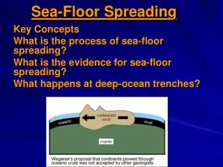
8. 3. Marine Magnetic Anomalies anomalies at sea calculated by subtracting main general field from detailed surface or satellite observations

9. Fig. 6 Magnetic anomalies (magnitude of total field) in the North Atlantic Ocean. Yellow box shows location of detailed region on the Reykjanes Ridge south of Iceland

10. Fig. 7 Location of the Reykjanes Ridge, SW of Iceland. The area of Fig. 8 is indicated by the box. Fig. 8 Magnetic anomalies near the crest of the Reykjanes Ridge. Red/yellow areas represent positive anomalies, blue/green areas negative anomalies. Fig. 9 Profiles of geomagnetic anomaly across the Reykjanes Ridge projected on lines at right angles to the ridge. A indicates the axis of the ridge.

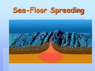
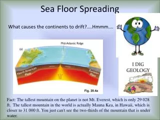
11. Fig. 10 Sea-floor spreading formation of magnetic anomalies. As magma is formed beneath mid-ocean ridges it rises. As it cools and solidifies to form the oceanic crust it is magnetized in the direction of the Earth’s magnetic field (a). As the plates separate and move this crust away from the spreading centre, new crust is formed with reversed and normal polarities during subsequent reversals of the field (b and c). The crust then becomes a tape recorder of the magnetic field reversals. Fig. 11 Models of the field reversals are made by comparing theoretical calculations of the field based on an assumed block model of field reversals with actual observations of magnetic profiles. By comparing models for various ridges a best fit sequence of reversals is determined. This sequence has been modified numerous times as new data is collected with improved resolution. This analysis only determines the anomaly identification relative to the distance from the spreading axis. Dates for the reversals must be determined independently. • Vine-Matthews-Morley hypothesis: • magma from mantle cools as it ascends beneath mid-ocean ridges • once cooled does not change so yields tape recording of past reversals • see following link for animation

12. Fig. 12 The acquisition of thermo-remanent magnetization (TRM). The acquisition of partial TRM (PTRM) acquiredover successive temperature intervals as the rock cools add up to give the total TRM curve. • Thermal Remanent Magnetism (TRM) • Magnetic field induced in upper crust as it cools through Curie point • Produced by Ferromagnetic Effect • Aligning of magnetic moments within regions creating a permanent field • Titanomagnetites - typical ferromagnetic minerals in basalt Fig. 13 FeO-TiO2-Fe2O3 ternary system of ferro-magnetic minerals in basalt, showing the principal solid solution series (solid lines). The dashed lines are some lines of constant Fe:Ti ratio along which oxidation may proceed in the direction of the arrows.

13. 4. Magnetic Stratigraphy

14. Fig. 14 Location of magnetic anomaly isochrons in the world’s oceans.

15. 2 cm/yr Fig. 15 Sites drilled during leg 3 of the Deep-Sea Drilling Program. Correlation between magnetic anomalies and age Fig. 16 The age of the oldest sediment drilled at each site plotted against the distance of the site from the spreading centre. All sites, except for sites 17 and 18, were drilled to the west of the ridge axis. The line is plotted for a constant spreading rate of 2 cm/yr. Basement was not reached at site 21. Fig. 17 The distance to a given anomaly in the South Atlantic versus distance to the same anomaly in the South Indian, North Pacific and South Pacific oceans. Numbers on right refer to anomaly numbers. In this manner, dates can be determined for other regions based on the drilling results for the South Atlantic.

16. Magnetic Stratigraphy • combination of reversals and dates yield polarity time scale • correlation w/ other geologic time scales • updated to include new reversals and improved ages • used to date ocean basins at present and to determine geological history of ocean spreading Fig. 18 Geomagnetic polarities (numbers) and geologic time scale for the Jurassic to recent times. Note the long periods of normal polarity for much of the Cretaceous and early Jurassic periods. Dates in millions of years before present (Ma).

17. Fig. 19 Crustal Age of the Ocean Basins Max age of oceans < 200 Ma which represents < 4% of Earth’s age

18. Fig. 20 Magnetic anomaly reconstructions of the continents and oceans from chron M 17 to 3A.

19. Web Sites: Reading List: Sharma, Geophysical Methods in Geology, ch. 4 pp. 155-189 sharma_ch4.pdf Fowler, The Solid Earth, ch. 3 and pp. 254-260 ch 7 fowler_ch3.pdf • WHOI Deeptow Magnetics Group • Digital Isochrons of the World's Ocean Floor