Download
1 / 27
270 likes | 282 Views
Learn about the gene finding task and the trade-off between predictive value and parameter uncertainty in choosing the order of a Markov model. Discover how interpolated Markov models can be used to locate genes in DNA sequences.

E N D
Interpolated Markov Models for Gene Finding BMI/CS 776 www.biostat.wisc.edu/bmi776/ Spring 2018 Anthony Gitter gitter@biostat.wisc.edu These slides, excluding third-party material, are licensed under CC BY-NC 4.0 by Mark Craven, Colin Dewey, and Anthony Gitter
Goals for Lecture Key concepts • the gene-finding task • the trade-off between potential predictive value and parameter uncertainty in choosing the order of a Markov model • interpolated Markov models
The Gene Finding Task • Given: an uncharacterized DNA sequence • Do: locate the genes in the sequence, including the coordinates of individual exons and introns
Sources of Evidence for Gene Finding • Signals: the sequence signals (e.g. splice junctions) involved in gene expression • Content: statistical properties that distinguish protein-coding DNA from non-coding DNA • Conservation: signal and content properties that are conserved across related sequences (e.g. orthologous regions of the mouse and human genome)
Gene Finding: Search by Content • Encoding a protein affects the statistical properties of a DNA sequence • some amino acids are used more frequently than others (Leu more prevalent than Trp) • different numbers of codons for different amino acids (Leu has 6, Trp has 1) • for a given amino acid, usually one codon is used more frequently than others • this is termed codon preference • these preferences vary by species
Codon Preference in E. Coli AA codon /1000 ---------------------- Gly GGG 1.89 Gly GGA 0.44 Gly GGU 52.99 Gly GGC 34.55 Glu GAG 15.68 Glu GAA 57.20 Asp GAU 21.63 Asp GAC 43.26
G C T A C G G A G C T T C G G A G C C G A T G C C T C G A A G C C T C G Reading Frames • A given sequence may encode a protein in any of the six reading frames
G T T AT G G C T • • • T C G T G A T T Open Reading Frames (ORFs) • An ORF is a sequence that • starts with a potential start codon • ends with a potential stop codon, in the same reading frame • doesn’t contain another stop codon in-frame • and is sufficiently long (say > 100 bases) • An ORF meets the minimal requirements to be a protein-coding gene in an organism without introns
reading frame G C T A C G G A G C T T C G G A G C G C T A C G G is in 3rd codon position C T A C G G G is in 1st position T A C G G A A is in 2nd position Markov Models & Reading Frames • Consider modeling a given coding sequence • For each “word” we evaluate, we’ll want to consider its position with respect to the reading frame we’re assuming • Can do this using an inhomogeneous model
Inhomogeneous Markov Model • Homogenous Markov model: transition probability matrix does not change over time or position • InhomogenousMarkov model: transition probability matrix depends on the time or position
now predict it given more history “…can you___” Higher Order Markov Models • Higher order models remember more “history” • Additional history can have predictive value • Example: • predict the next word in this sentence fragment “…you__”(are, give, passed, say, see, too, …?) “…say can you___” “…oh say can you___” YouTube
AAAAA CTACA CTACC CTACG CTACT GCTAC TTTTT A Fifth Order Inhomogeneous Markov Model start position 2
AAAAA AAAAA CTACA CTACA CTACC CTACC CTACG CTACG CTACT CTACT GCTAC GCTAC TTTTT TTTTT A Fifth Order Inhomogeneous Markov Model AAAAA CTACA start TACAA Trans. to states in pos. 2 TACAC TACAG TACAT TTTTT position 2 position 3 position 1
Selecting the Order of a Markov Model • But the number of parameters we need to estimate grows exponentially with the order • for modeling DNA we need parameters for an nth order model • The higher the order, the less reliable we can expect our parameter estimates to be • Suppose we have 100k bases of sequence to estimate parameters of a model • for a 2nd order homogeneous Markov chain, we’d see each history 6250 times on average • for an 8th order chain, we’d see each history ~ 1.5 times on average
Interpolated Markov Models • The IMM idea: manage this trade-off by interpolating among models of various orders • Simplelinear interpolation: • where
Interpolated Markov Models • We can make the weights depend on the history • for a given order, we may have significantly more data to estimate some words than others • Generallinear interpolation λ is a function of the given history
The GLIMMER System[Salzberg et al., Nucleic Acids Research, 1998] • System for identifying genes in bacterial genomes • Uses 8th order, inhomogeneous, interpolated Markov models
Let be the number of times we see the history in our training set IMMs in GLIMMER • How does GLIMMER determine the values? • First, let’s express the IMM probability calculation recursively
IMMs in GLIMMER • If we haven’t seen more than 400 times, then compare the counts for the following: nth order history + base (n-1)th order history + base • Use a statistical test to assess whether the distributions of depend on the order
IMMs in GLIMMER nth order history + base (n-1)th order history + base • Null hypothesis in test: distribution is independent of order • Define • If is small we don’t need the higher order history
IMMs in GLIMMER • Putting it all together where
IMM Example ACGA 25 ACGC 40 ACGG 15 ACGT 20 ___ 100 CGA 100 CGC 90 CGG 35 CGT 75 ___ 300 GA 175 GC 140 GG 65 GT 120 ___ 500 • Suppose we have the following counts from our training set χ2 test: d = 0.140 χ2 test: d = 0.857 λ3(ACG) = 0.857 × 100/400 = 0.214 λ2(CG) = 0 (d < 0.5, c(CG) < 400) λ1(G) = 1 (c(G) > 400)
IMM Example (Continued) • Now suppose we want to calculate
Gene Recognition in GLIMMER • Essentially ORF classification • For each ORF • calculate the probability of the ORF sequence in each of the 6 possible reading frames • if the highest scoring frame corresponds to the reading frame of the ORF, mark the ORF as a gene • For overlapping ORFs that look like genes • score overlapping region separately • predict only one of the ORFs as a gene
Gene Recognition in GLIMMER JCVI ORF meeting length requirement Low scoring ORF High scoring ORF
GLIMMER Experiment • 8th order IMM vs. 5th order Markov model • Trained on 1168 genes (ORFs really) • Tested on 1717 annotated (more or less known) genes
GLIMMER Results TP FN FP & TP? • GLIMMER has greater sensitivity than the baseline • It’s not clear whether its precision/specificity is better