Download
1 / 39
390 likes | 639 Views
Adiabatic theorem and Berry phase. Consider Evolution of a system when adiabatic theorem holds (discrete spectrum, no degeneracy, slow changes). 1. 1. To find the Berry phase, we start from the expansion on instantaneous basis.

E N D
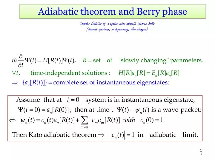
Adiabatic theorem and Berry phase Consider Evolution of a system when adiabatic theorem holds (discrete spectrum, no degeneracy, slow changes) 1 1
To find the Berry phase, we start from the expansion on instantaneous basis Negligible because second order (derivative is small, in a small amplitude) 2
Now, scalar multiplication by an removes all other states! 3 3 Professor Sir Michael Berry
C 4
VectorPotentialAnalogy One naturally writes introducing a sort of vector potential (which depends on n, however). The gauge invariance arises in the familiar way, that is, if we modify the basis with and the extra term, being a gradient in R space, does not contribute. The Berry phase is real since We prefer to work with a manifestly real and gauge independent integrand; going on with the electromagnetic analogy, we introduce the field as well, such that 5
The last term vanishes, To avoid confusion with the electromagnetic field in real space one often speaks about the Berry connection and the gauge invariant antisymmetric curvature tensor with components 6
Formula for the curvature The m,n indicesrefertoadiabaticeigenstatesof H ; the m=ntermactuallyvanishes (vectorproductof a vectorwithitself). Itisusefultomake the Berry conectionsappearinghere more explicit, bytaking the gradientof the Schroedingerequation in parameterspace: Taking the scalar product with an orthogonal am A nontrivial topology of parameter space is associated to the Berry phase, and degeneracies lead to singular lines or surfaces 7
Quantum Transport in nanoscopic devices Ballistic conduction - no resistance If all lengths are small compared to the electron mean free path the transport is ballistic (no scattering, no Ohm law). This occurs in Carbon Nanotubes (CNT) , nanowires, Graphene,… A graphene nanoribbon field-effect transistor (GNRFET) from Wikipedia This makes problems a lot easier (if interactions can be neglected). In macroscopic conductors the electron wave functions that can be found by using quantum mechanics for particles moving in an external potential lose coherence when travelling a mean free path because of scattering . Dissipative events obliterate the microscopic motion of the electrons . In ballistic transport the quantum propertes of the electrons are revealed.
W left electrode right electrode Ballistic conductor between contacts Fermi level left electrode Fermi level right electrode
W left electrode right electrode For transport across a junction with M conduction modes, i.e. bands of the unbiased hamiltonian at the Fermi level one measures a finite conductivity. If V is the bias, eV= difference of Fermi levels across the junction, This quantum can be measured. 10
B.J. Van Wees experiment (prl 1988) A negative gate voltage depletes and narrows down the constriction progressively Conductance is indeed quantized in units 2e2/h 11
Current-Voltage Characteristics: Landauer formula (1957) Rolf Landauer Stutgart 1927-New York 1999 Phenomenological description of conductance at a junction
Quantum system J More general formulation, describing the propagation inside a device. Let represent leads with Fermi energy EF, Fermi function f(e), density of states r(e) bias 13
Quantum system J current-voltage characteristic J(V) This scheme was introduced phenomenologically by Landauer but later confirmed by rigorous quantum mechanical calculations for non-interacting models. 14
device J Microscopic current operator 16
Pseudo-Hamiltonian Approach device =pseudo-Hamiltonian connecting left and right Traditional partitioned approach (Caroli, Feuchtwang): fictitious unperturbed biased system with left and right parts that obey special boundary conditions this is a perturbation (to be treated at all orders = left-right bond Drawback: separate parts obey strange bc and do not exist. 17
U=1 current Simple junction-Static current-voltage characteristics J 1 U=0 (no bias) U=2 -2 2 Left wire DOS 0 Right wire DOS no current no current
Meir-WinGreen Formula Quantum dot U Consider a quantum dot ( a nano conductor with size of angstroms, modeled for example by an Anderson model) connected with wires where L,R refers to the left and right electrodes. Due to small size, charging energy U is important. If one electron jumps into it, the arrival of a second electron is hindered (Coulomb blockade)
Quantum dot U and the like, even in the presence of the bias. Meir and WinGreen in 1992 have shown, using the Keldysh formalism, that the current through the quantum dot is given by This has been used for weak V also in the presence of strong U. 21
General partition-free framework and rigorousTime-dependentcurrent formula Partitioned approach has drawbacks: it is different from what is done experimentally, and L and R subsystems not physical, due to specian boundary conditions. It is best to include time-dependence! 22
Time-dependent Quantum Transport device J System is in equilibrium until at time t=0 blue sites are shifted to V and J starts 23
General formulation for independent-electron problems Equation Of Motion for time-ordered GF EOM for retarded (advanced) GF EOM is the same, but initial conditions differ
Initial conditions for time-ordered: GF Initial conditions for retarded: GF With H constant up to t=0, here is the solution for t>0,t’>0 (Blandin, Nourtier, Hone (1976) had derived this formula by the Keldysh formalism in a paper on atom-surface scattering
Note: Occupationnumbersreferto H before the timedependencesets in! System remembersinitialconditions! This allows to write a rigorous time-dependent current formula
Current-Voltage characteristics In the 1980 paper I have shown how one can obtain the current-voltage characteristics by a long-time asyptotic development. Recently Stefanucci and Almbladh have shown that the characteristics for non-interacting systems agree with Landauer
Long-Time asymptotics and current-voltage characteristics are the same as in the earlier partitioned approach
In addition one can study transient phenomena Transient current asymptote Current in the bond from site 0 to -1
M. Cini E.Perfetto C. Ciccarelli G. Stefanucci and S. Bellucci, PHYSICAL REVIEW B 80, 125427 2009
M. Cini E.Perfetto C. Ciccarelli G. Stefanucci and S. Bellucci, PHYSICAL REVIEW B 80, 125427 2009
G. Stefanucci and C.O. Almbladh (Phys. Rev 2004) extended to TDDFT LDA scheme TDDFT LDA scheme not enough for hard correlation effects: Josephson effect would not arise Keldysh diagrams should allow extension to interacting systems, but this is largely unexplored. Retardation + relativistic effects totally to be invented!
Pumping in 1d insulator with adiabatic perturbation periodic in space and time H(t+T)=H(t) (Thouless Phys. Rev. B (1983) ) A B A B A B A B A B A B Perturbation such that Fermi level remains within gap
Niu and Thouless have shown that weak perturbations, interactions and disorder cannot change the integer.
length along wire length along wire length along wire length along wire back to phase 1 Two parameter pumping in 1d wire Example taken from P.W.Brouwer Phys. Rev.B 1998
Bouwer formulation for Two parameter pumping assuming linear response to parameters X1, X2 There is a clear connection with the Berry phase (see e.g. Di Xiao,Ming-Che-Chang, Qian Niu cond-mat 12 Jul 2009). The magnetic charge that produces the Berry magnetic field is made of quantized Dirac monopoles arising from degeneracy. The pumping is quantized.
time-periodic gate voltage Mono-parametric quantum charge pumping ( Luis E.F. Foa Torres PRB 2005) quantum charge pumping in an open ring with a dot embedded in one of its arms. The cyclic driving of the dot levels by a single parameter leads to a pumped current when a static magnetic flux is simultaneously applied to the ring. The direction of the pumped current can be reversed by changing the applied magnetic field. The response to the time-periodic gate voltage is nonlinear. The pumping is not adiabatic.No pumping at zero frequency. The pumping is not quantized.