Download
1 / 24
520 likes | 1.75k Views
Smart antenna. Smart antennas use an array of low gain antenna elements which are connected by a combining network . Smart antennas provide enhanced coverage through range extension , hole filling , and better building penetration . Smart antennas can improve system capacity .

E N D
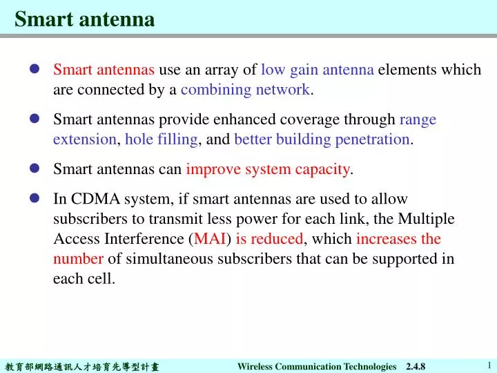
Smart antenna Smart antennas use an array of low gain antenna elements which are connected by a combining network. Smart antennas provide enhanced coverage through range extension, hole filling, and better building penetration. Smart antennas can improve system capacity. In CDMA system, if smart antennas are used to allow subscribers to transmit less power for each link, the Multiple Access Interference (MAI) is reduced, which increases the number of simultaneous subscribers that can be supported in each cell. 2.4.8
Smart antenna The array is frequently implemented as a linear equally spaced (LES), co-polarized, low gain elements, which are oriented in the same direction. For a plane wave incident on the array from direction , the difference in phase between the signal component incident on array element m and a reference element at the origin is where is the phase propagation factor and the term λ denotes the wavelengh. 2.4.8
Smart antenna A simple M-element LES antenna array is illustrated in Figure. 2.4.8
Smart antenna The baseband complex envelope representation of the array is shown in Figure. Each branch of the array has a weighting element, , which has both a magnitude and a phase associated with it. 2.4.8
Smart antenna Assume that all of the array elements are noiseless isotropic an-tennas which have uniform gain in all directions. With and , the signal received at antenna element m is where A is the arbitrary gain constant. The signal at the array output is The term is called the array factor. The array factor determines the ratio of the received signal available at the array output to the signal, , measured at the reference element, as a function of Direction-of-arrival. 2.4.8
Smart antenna By adjusting the set of weights, , it is possible to direct the maximum of the main beam of the array factor in any desired direction. To show how the weights can be used to change the antenna pattern of the array, let the mth weight be given by Then the array factor is 2.4.8
Smart antenna The array factor (in dB) is shown in Figure for . By varying a single parameter, , the beam can be steered to any desired direction. 2.4.8
Smart antenna Define the weight vector as where the superscript H represents the Hermitian transpose. The signal from each antenna element are grouped in a data vector Then the array output can be expressed as The vector is called the steering vector. The steering vector describes the phase of the signal available at each antenna element relative to the phase of the signal at the reference element 0. 2.4.8
Smart antenna In an adaptive array, the weight vector is adjusted to maximize the quality of the signal that is available to the demodulator. 2.4.8
MMSE for smart antenna In optimal beamforming techniques, a weight vector is determined which minimizes a cost function. This cost function is inversely associated with the quality of the signal at the array output, so that when the cost function is minimized, the quality of the signal is maximized at the array output. A popular technique which has been applied extensively in communication systems is the Minimum Mean Square Error (MMSE). In this technique, the square of the difference between the array out, , and , a locally generated estimate of the desired signal for the kth subscriber, is minimized by finding an appropriate weight vector, . 2.4.8
MMSE for smart antenna MMSE solutions are posed in terms of ensemble averages and produce a single weight vector, , which is optimal over the ensemble of possible realizations of the stationary environment. In the MMSE approach, the cost function to be minimized is where and where is the sampling period. Setting the gradient of the cost function equal to zero, we find that the solution for is where is the correlation matrix of the data vector and is the cross-correlation between the data vector and the desired signal. 2.4.8
Simulation of MMSE for smart antenna Fig. shows the array patterns achieved when three components are incident on a eight element LES array with half wavelength spacing. 2.4.8
Simulation of MMSE for smart antenna In the above plot, three signals are incident on the array, one Signal-of-Interest (SOI) from and two Signal-Not-of-Interests (SNOI) from and . It can be seen that the array forms deep nulls in the directions of each SNOI component to reduce the effects of interferences. The optimum MMSE approach is derived for optimal spatial filtering, there is a disadvantage that it must be given a desired signal, . Some optimal spatial filtering, such as (1) the Max SNR approach which maximizes the actual signal-to-noise ratio at the array output and (2) the Linearly Constrained Minimum Variance (LCMV) approach, require knowledge of the Direction-of-Arrival (DOA) of the desired signal [10]. 2.4.8
DOA estimation The array-based DOA estimation techniques are broadly divided into four different types: conventional techniques, subspace based techniques, maximum likelihood techniques and the integrated techniques. In this section, we only introduce the MUSIC method , which belongs to the subspace based techniques. 2.4.8
DOA estimation - MUSIC Subspace based methods are high resolution sub-optimal techniques which exploit the eigen structure of the input data matrix. A technique proposed by Schmidt is called Multiple Signal Classification (MUSIC) algorithm. The MUSIC algorithm is a high resolution multiple signal classification technique based on exploiting the eigenstructure of the input covariance matrix. MUSIC is a signal parameter estimation algorithm which provides information about the number of incident signals, DOA of each signal, strengths and cross correlations between incident signals, noise power, etc. 2.4.8
DOA estimation - MUSIC The development of the MUSIC algorithm is based on a geometric view of the signal parameter estimation problem. If there are D signals incident on the array, the received input data vector at an M-element array can be expressed as a linear combination of the D incident waveforms and noise. That is, or where is the vector of incident signals, is the noise vector, and is the array steering vector corresponding to the DOA of the jth signal. 2.4.8
DOA estimation - MUSIC In geometric terms, the received vector and the steeling vector can be visualized as vectors in M dimensional space. The input covariance matrix can be expressed as where is the signal correlation matrix . The eigenvalues of are the values, , such that Then we can rewrite this as 2.4.8
DOA estimation - MUSIC By additional analysis [10], it shows that the eigenvectors of the covariance matrix belong to either of the two orthogonal subspaces, called the principal eigen subspace (signal space) and the non-principal eigen subspace (noise subspace). The steering vectors corresponding to the DOA lie in the signal subspace and are hence orthogonal to the noise subspace. By searching through all possible array steering vectors to find those which are perpendicular to the space spanned by the non-principal eigenvectors, the DOAs can be determined. 2.4.8
DOA estimation - MUSIC To search the noise subspace, we form a matrix containing the noise eigenvectors: Sincethe steering vectors corresponding to signal components are orthogonal to the noise subspace eigenvector, for corresponding to the DOA of a incident component. Then the DOAs of the multiple incident signals can be estimated by locating the peaks of a MUSIC spactial spectrum given by The largest peaks in the MUSIC spectrum correspond to the DOA of the signals impinging on the array. 2.4.8
DOA estimation – modified MUSIC Fig. shows an example how to combine the MUSIC algorism and the smart antennainCDMA system,we call it as modified MUSIC. 2.4.8
DOA stimation – modified MUSIC simulation Table shows the related parameters in the simulation. 2.4.8
DOA estimation – modified MUSIC simulation Figs. show the comparison between the resolution performance of the modified MUSIC and the MODAS. As seen clearly from the plot, MUSIC has a sharp peak directing to . The Delay-and-Sum method, also referred to as the classical beamformer method, is one of the simplest techniques for DOA estimation. The MODAS is a modified form the Delay-and-Sum algorism. 2.4.8
DOA estimation – modified MUSIC simulation Fig. show BER comparisons between three methods: MMSE, modified MUSIC and MODAS. It can be seen that the three methods perform as well and all have an obvious power gain. In right-side Fig., the performance is poor than in the left-side, since the MAI for N=15 is larger than left-side for N=3. 2.4.8
DOA estimation – modified MUSIC simulation Figs. show BER comparisons for different processing gain. From Figs. we see that the performance for PG=127 is much better than PG=31. We conclude that the smart antenna can obviously enhance the BER performance of CDMA systems. 2.4.8