Download
1 / 4
40 likes | 44 Views
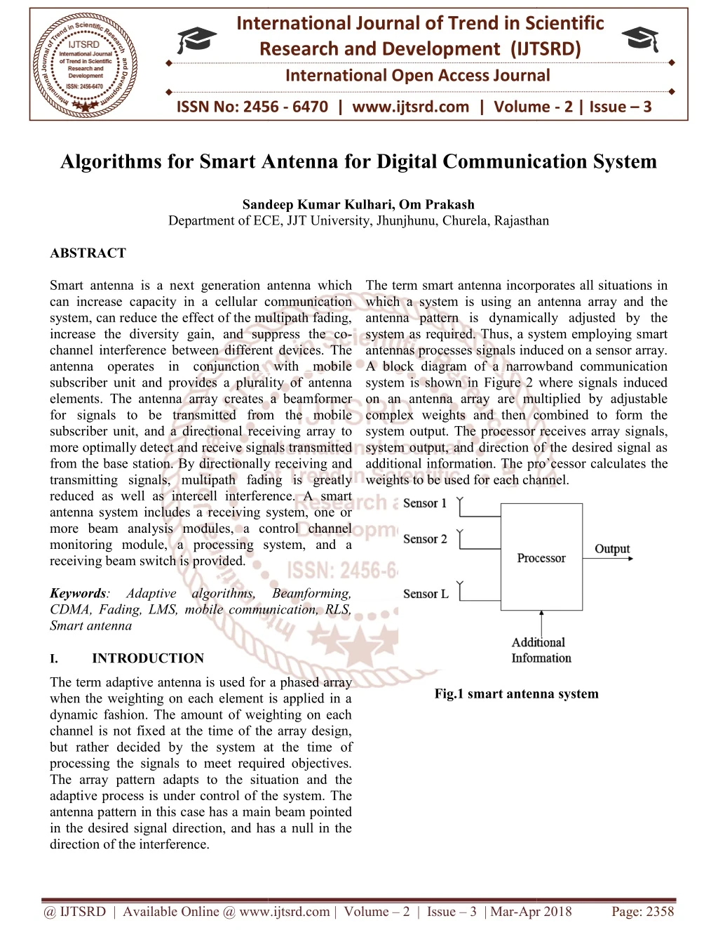
Smart antenna is a next generation antenna which can increase capacity in a cellular communication system, can reduce the effect of the multipath fading, increase the diversity gain, and suppress the co channel interference between different devices. The antenna operates in conjunction with mobile subscriber unit and provides a plurality of antenna elements. The antenna array creates a beamformer for signals to be transmitted from the mobile subscriber unit, and a directional receiving array to more optimally detect and receive signals transmitted from the base station. By directionally receiving and transmitting signals, multipath fading is greatly reduced as well as intercell interference. A smart antenna system includes a receiving system, one or more beam analysis modules, a control channel monitoring module, a processing system, and a receiving beam switch is provided. Sandeep Kumar Kulhari | Om Prakash "Algorithms for Smart Antenna for Digital Communication System" Published in International Journal of Trend in Scientific Research and Development (ijtsrd), ISSN: 2456-6470, Volume-2 | Issue-3 , April 2018, URL: https://www.ijtsrd.com/papers/ijtsrd12785.pdf Paper URL: http://www.ijtsrd.com/engineering/electronics-and-communication-engineering/12785/algorithms-for-smart-antenna-for-digital-communication-system/sandeep-kumar-kulhari<br>

E N D
International Research Research and Development (IJTSRD) International Open Access Journal ntenna for Digital Communication System International Journal of Trend in Scientific Scientific (IJTSRD) International Open Access Journal ISSN No: 2456 ISSN No: 2456 - 6470 | www.ijtsrd.com | Volume 6470 | www.ijtsrd.com | Volume - 2 | Issue – 3 Algorithms for Smart A Algorithms for Smart Antenna for Digital Communication System Sandeep Kumar Kulhari, Om Prakash Department of ECE, of ECE, JJT University, Jhunjhunu, Churela, Rajasthan Sandeep Kumar Kulhari, Om Prakash Churela, Rajasthan The term smart antenna incorporates all situations in which a system is using an antenna array and the antenna pattern is dynamically adjusted by the system as required. Thus, a system employing smart antennas processes signals induc A block diagram of a narrowband communication system is shown in Figure 2 where signals induced on an antenna array are multiplied by adjustable complex weights and then combined to form the system output. The processor receives array system output, and direction of the desired signal as additional information. The pro weights to be used for each channel. weights to be used for each channel. ABSTRACT Smart antenna is a next generation antenna which can increase capacity in a cellular communication system, can reduce the effect of the multipath fading, increase the diversity gain, and suppress the co channel interference between different devices. The antenna operates in conjunction with mobile subscriber unit and provides a plurality of antenna elements. The antenna array creates a beamformer for signals to be transmitted from the mobile subscriber unit, and a directional receiving array to more optimally detect and receive signals transmitted from the base station. By directionally receiving and transmitting signals, multipath fading is greatly reduced as well as intercell interference. A smart antenna system includes a receiving system, one or more beam analysis modules, a control channel monitoring module, a processing system, and a receiving beam switch is provided. Keywords: Adaptive algorithms, Beamforming, CDMA, Fading, LMS, mobile communication, RLS, Smart antenna I. INTRODUCTION Smart antenna is a next generation antenna which can increase capacity in a cellular communication system, can reduce the effect of the multipath fading, increase the diversity gain, and suppress the co- channel interference between different devices. The ntenna operates in conjunction with mobile subscriber unit and provides a plurality of antenna elements. The antenna array creates a beamformer for signals to be transmitted from the mobile subscriber unit, and a directional receiving array to ly detect and receive signals transmitted from the base station. By directionally receiving and transmitting signals, multipath fading is greatly reduced as well as intercell interference. A smart antenna system includes a receiving system, one or m analysis modules, a control channel monitoring module, a processing system, and a The term smart antenna incorporates all situations in which a system is using an antenna array and the antenna pattern is dynamically adjusted by the system as required. Thus, a system employing smart antennas processes signals induced on a sensor array. A block diagram of a narrowband communication system is shown in Figure 2 where signals induced on an antenna array are multiplied by adjustable complex weights and then combined to form the system output. The processor receives array signals, system output, and direction of the desired signal as additional information. The pro`cessor calculates the : Adaptive algorithms, Beamforming, CDMA, Fading, LMS, mobile communication, RLS, The term adaptive antenna is used for a phased array when the weighting on each element is applied in a dynamic fashion. The amount of weighting on each channel is not fixed at the time of the array design, but rather decided by the system at the time of processing the signals to meet required objectives. The array pattern adapts to the situation and the adaptive process is under control of the system. The antenna pattern in this case has a main beam pointed in the desired signal direction, and has a null in the direction of the interference. antenna is used for a phased array Fig.1 smart antenna system Fig.1 smart antenna system when the weighting on each element is applied in a dynamic fashion. The amount of weighting on each channel is not fixed at the time of the array design, but rather decided by the system at the time of als to meet required objectives. The array pattern adapts to the situation and the adaptive process is under control of the system. The antenna pattern in this case has a main beam pointed in the desired signal direction, and has a null in the @ IJTSRD | Available Online @ www.ijtsrd.com @ IJTSRD | Available Online @ www.ijtsrd.com | Volume – 2 | Issue – 3 | Mar-Apr 2018 Apr 2018 Page: 2358
International Journal of Trend in Scientific International Journal of Trend in Scientific Research and Development (IJTSRD) ISSN: 2456 Research and Development (IJTSRD) ISSN: 2456-6470 of factors like the aperture of the array determine the that the array can achieve, similarly the number of elements determine the degree of of factors like the aperture of the array determine the maximum gain that the array can achieve, similarly the number of elements determine the degree of freedom. III. ADAPTIVE PROCESSING Adaptive processing represents a significant part of the subject of statistical signal processing upon which they are founded. Many differe algorithms are here. We are discussing some linear adaptive algorithms in this article A.The LMS Algorithms The LMS adaptive algorithm is a practical method for finding close approximate solutions to the Wiener-Hopf equations which is not dependent on priori knowledge of the autocorrelation of the input process and the cross correlation between the input and the desired output, steepest gradient descent as defined by { ] [ ] 1 [ e E k w k w Where is a small positive gain factor that controls stability and rate of convergence. The true gradient of the mean square error function, ]} [ { e E can be estimated by an instantaneous can be estimated by an instantaneous ADAPTIVE PROCESSING Adaptive processing represents a significant part of the subject of statistical signal processing upon which they are founded. Many different adaptive algorithms are here. We are discussing some linear adaptive algorithms in this article Fig. 2 Block diagram of a communication system using an antenna array. Fig. 2 Block diagram of a communication system array. II. Smart antenna uses an array of low gain antenna elements which are connected by a combining network. The spacing between the array elements is small enough that there is no amplitude variation between the signals received at different elements, there is no mutual coupling between the elements and the bandwidth of the signal incident on the array is small as compared with the carrier frequency. In working with array antenna it is convenient to use the vector notation (weight vector) which is defined as 1 0 .. .......... , M w w w w Where H is the Hermitian transpose. The signal from each antenna element are grouped in a data vector x t x t x x . )......... ( , 1 0 Then the array output y (t) is defined as ) ( ) ( t x w t y The array factor in the direction (θ,φ), where θ is the angle of elevation and φ is the azimuthal angle of plane wave incident on antenna array, is defined as ) , ( ) , ( a w f Where is the steering vector in direction ) , ( The steering vector of the signal available at each array element relative to the phase of signal at the reference element. The steering vector is a a )......... , ( , 1 ) , ( 1 ) , ( is called the Direction of Arrival (DOA) of the plane wave. In general the utility of an antenna array is determined by a number utility of an antenna array is determined by a number The LMS adaptive algorithm is a practical method for finding close approximate solutions to the equations which is not dependent on a knowledge of the autocorrelation of the input process and the cross correlation between the input and the desired output, steepest gradient descent as SMART ANTENNA TECHNOLOGY SMART ANTENNA TECHNOLOGY Smart antenna uses an array of low gain antenna elements which are connected by a combining network. The spacing between the array elements is small enough that there is no amplitude variation at different elements, between the elements 2k [ k ]} (6) mall positive gain factor that and the bandwidth of the signal incident on the array is small as compared with the carrier frequency. In working with array antenna it is convenient to use the vector) which is defined as controls stability and rate of convergence. The true gradient of the mean square error function, 2k 2k e [ ] (1) 1 gradient by assuming that single error sample, is an adequate estimate of the mean square error. The Widrow-Hoff LMS algorithm can be defined as 2 ] [ ] 1 [ e k w k w Where: = learning rate parameter. ] [k e = error (desired output - actual output). ] [k x = vector at instance k. ] [k w = weight vector at instance The LMS has following important properties it can be used to solve the wiener hopf equation without finding matrix inversion it is capable to delivering high performance during the adaptation process it is stable and robust for a variety of signal condition , the square of a Where H is the Hermitian transpose. The signal from each antenna element are grouped in a data vector single error sample, is an adequate estimate of the T Hoff LMS algorithm can be defined as [k ( t ) (2) M 1 [ k ] x x ] (7) Then the array output y (t) is defined as H (3) = learning rate parameter. The array factor in the direction (θ,φ), where θ is the angle of elevation and φ is the azimuthal angle of plane wave incident on antenna array, is defined as actual output). , the tap t T x , x ( t )......... . x ( t ) 0 1 p 1 H (4) t ( a , ) T w , w ( t )......... w . ( t t) is the steering vector in direction the tap- 0 1 p 1 ( , ) ,describes the phase ,describes the phase weight vector at instance k. of the signal available at each array element relative to the phase of signal at the reference element. The The LMS has following important properties it can be used to solve the wiener hopf equation without finding matrix inversion it is capable to delivering high performance during the adaptation process it is stable and robust for a variety of signal T a ( , ) (5) M 1 The angle pair Arrival (DOA) of the plane wave. In general the is called the Direction of @ IJTSRD | Available Online @ www.ijtsrd.com @ IJTSRD | Available Online @ www.ijtsrd.com | Volume – 2 | Issue – 3 | Mar-Apr 2018 Apr 2018 Page: 2359
International Journal of Trend in Scientific International Journal of Trend in Scientific Research and Development (IJTSRD) ISSN: 2456 Research and Development (IJTSRD) ISSN: 2456-6470 it does not required the availability of autocorrelation matrix of the filter input and cross correlation between filter input and its desired signal. B.The Normalised LMS Algorithm The problem with LMS algorithms is that if the input vector magnitude is large the filter weights also change by a larger amount. It could be desirable to normalise this vector in some way. This algorithm is a variation of the constant-step-size LMS algorithm and uses a data dependent step size at each iteration. It avoids the need for estimating the eigenvalues of the correlation matrix. The algorithm normally has better convergence performance and less signal sensitivity compared to the normal LMS algorithm. In normalised LMS algorithm the input vector the desired response weights are given and we find the updated filter weights that minimise the squared Euclidean norm of the difference the constraint equation for NLMS is given by 2 ] [ ] 1 [ a T it does not required the availability of autocorrelation matrix of the filter input and cross correlation between filter input and its desired w [ n ] [ w [ n ], w [ n ]...... w w [ n ]] (10) 0 1 p 1 The error between the desired response at time the filter output for an input of coefficients at time n is defined by is defined by The error between the desired response at time k and the filter output for an input of x [k ] with the filter x The problem with LMS algorithms is that if the input is large the filter weights also change by a larger amount. It could be desirable to normalise this vector in some way. This algorithm is T e [ n , k ] d [ k ] w [ n ] [ k ] ](11) The error term (n ) for this can be defined by for this can be defined by size LMS algorithm ep size at each iteration. n 2 ( n ) ( n , k ) e [ n , k ] the need for estimating the eigenvalues of the correlation matrix. The algorithm normally has better convergence performance and less signal sensitivity compared to the normal LMS algorithm. In normalised LMS algorithm the input vector k 0 n 2 w wT ( n , k ) d [ k ] [ n ] X [ k ] (12) k 0 IV. x [k ] , COMPARISON BETWEEN LMS AND RLS ALGORITHMS RLS ALGORITHMS COMPARISON BETWEEN LMS AND d [k ] and the current filter and the current filter w [k [ k w ] are given and we find the updated filter that minimise the squared Euclidean ] 1 ] 1 ] . The weight update The weight update w [ k [ w w [k ] subject to ] 1 d [ k ] w [ k x k e [ k ] w k w k 2x x [k ] ( x [ k ] ) (8) Where a > 0 C.Recursive Least Squares Estimation Recursive Least Squares (RLS) estimation is a special case of Kalman filtering. It is actually an extension of Least Square Estimation where the estimate of the coefficients of an optimum filter are updated using a combination of the previous set of coefficients and a new observation. In RLS we consider a zero mean complex valued time series ..... 2 , 1 ], [ i k x and a corresponding set of desired filter responses . Vector samples from the time series are denoted as, k x k x k x ]...... 1 [ ], [ [ ] [ and the coefficients of a time-varying FIR filter at time n are denoted as, Figure 3: PN(w(n)) vs. the iteration number (n)) vs. the iteration number In figure 3, A linear array of ten elements with half wavelength spacing is assumed. The variance of uncorrelated noise present on each element is assumed to be equal to 0.1; two interference sources are assumed to be present. The first interference falls in the main lobe of the conventional array pattern and makes an angle of 98° with the line of the array. The power of this interference is taken to be 10 dB more than the uncorrelated noise power. The second interference makes an angle of 72° with the line of the array and falls in the first side conventional pattern. The power of this interference is 30 dB more than the uncorrelated noise power. The look direction is broadside to the array. For the improved LMS algorithm the gradient step size μ is taken to be equal to 0.00005 and for the RLS algorithm ε0 is taken to be 0.0001. According to is taken to be 0.0001. According to linear array of ten elements with half- wavelength spacing is assumed. The variance of uncorrelated noise present on each element is assumed to be equal to 0.1; two interference sources are assumed to be present. The first interference falls be of the conventional array pattern and makes an angle of 98° with the line of the array. The power of this interference is taken to be 10 dB more than the uncorrelated noise power. The second interference makes an angle of 72° with the line of and falls in the first side-lobe of the conventional pattern. The power of this interference is 30 dB more than the uncorrelated noise power. The look direction is broadside to the array. Recursive Least Squares Estimation Recursive Least Squares (RLS) estimation is a filtering. It is actually an extension of Least Square Estimation where the estimate of the coefficients of an optimum filter are updated using a combination of the previous set of coefficients and a new observation. In RLS we valued time series and a corresponding set of desired . Vector samples from the time d [k ] T x [ k p 1 ]] (9) For the improved LMS algorithm the gradient step be equal to 0.00005 and for the varying FIR filter at @ IJTSRD | Available Online @ www.ijtsrd.com @ IJTSRD | Available Online @ www.ijtsrd.com | Volume – 2 | Issue – 3 | Mar-Apr 2018 Apr 2018 Page: 2360
International Journal of Trend in Scientific Research and Development (IJTSRD) ISSN: 2456-6470 the figure 3, for a weak signal the RLS algorithm performs better than the improved algorithm. REFERENCES 1.Godara, L.C., IEEE Trans. Antennas Propagat., 38, 1631–1635, 1990. 2.J. C. Liberti, Jr. and T.S. Rappaport, Analytical results for reverse improvements in CDMA cellular communication systems employing adaptive antennas, IEEE Trans. on Vehicular Technology, vol. 43, no. 3, pages 680-690, Aug. 1994 3.J. G. Proakis. Digital Communications. McGraw- Hill Book Company, Polytechnic Institute of New York, second edition, 1989. 4.J. C. Liberti and T. S. Rappaport, Smart antennas for wireless communications, Prentice Hall, 1999. 5.H. J. Sing, J. R. Crux, and Y. Wang, “Fixed Multibeam Antennas Versus Adaptive Arrays for CDMA Systems,” IEEE Vehicular Technology Conference, pp. 27-31, September 1999. 6.J. S. Thompson, P. M. Grant, and B. Mulgrew, “Smart Antenna Arrays for CDMA Systems,” IEEE Personal Communications, pp. 16-25, October 1996. 7.Y. S. Song and H. M. Kwon, “Analysis of a Simple Smart Antenna for CDMA Wireless Communications,” IEEE Vehicular Technology Conference, pp. 254-258, May 1999. 8.G. Dolmans and L. Leyten, “Performance Study of an Adaptive Dual Antenna Handset for Indoor Communications,” IEE Microwaves, Antennas and Propagation, Vol. 146, No. 2, pp. 138-1444, April 1999. 9.Ottersten, B. and Kailath, T., Direction-of-arrival estimation for wide-band signals using the ESPRIT algorithm, IEEE Trans. Acoust. Speech Signal Process., 38, 317–327, 1990. 10.Nagatsuka, M., et al., Adaptive array antenna based on spatial spectral estimation using maximum entropy method, Commn., E77-B, 624–633, 1994. SANDEEP KUMAR KULHARI (san.kulhari@gmail.com ) received a B.E. degree in Electronics & Communication from the University of Rajasthan, Jaipur in 2003, and an M.Tech. degree from the Malviya National Institute of Technology Jaipur (MNIT Jaipur) in Digital Communication in the year 2007. He is pursuing his PhD degree from Shri JJT University, Jhunjhunu. He is presently employed with a leading Engineering Institute at a Top management level. He has worked in various capacities and has been actively involved in major switching and transmission projects. His area of interest is wireless multimedia communications, wireless broadband communications & fixed mobile convergence fields. Dr OM PRAKASH (om4096@gmail.com) He received the AMIETE degree in electronics and telecom engineering from IETE, New Delhi, India, in 2008, and the M. Tech. degree in Instrumentation and Control engineering from Sant Longowal Institute of Engg & Technology Longowal, Punjab, India in 2010 and the PhD degree in electronics and communication engineering from Shri Jagdish Prasad Jhabarmal Tibrewala University, Rajasthan, India in 2015. At present he is working with Malla Reddy Institute of Engineering & Technology, Hyderabad, India in the capacity of Professor in electronics Department. He is the author of more than 25 journal and conference papers. His fields of interest include power system optimization, Image signal processing, Antenna design and wireless communication. He is the Member of Scientific and Industrial Research Organization, IETE, Delhi Association of Engineers (IAENG), Hong Kong. channel performance and communication Proceedings of and International IEICE Trans. @ IJTSRD | Available Online @ www.ijtsrd.com | Volume – 2 | Issue – 3 | Mar-Apr 2018 Page: 2361