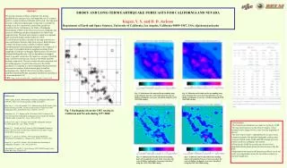
Abstract Since 1977 we have developed statistical short- and long-term earthquake forecasts to predict earthquake rate p

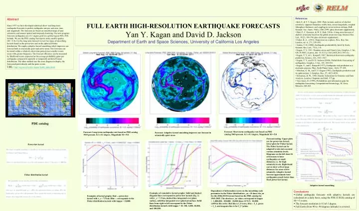
1. AbstractSince 1977 we have developed statistical short- and long-term earthquake forecasts to predict earthquake rate per unit area, time, and magnitude. The forecasts are based on smoothed maps of past seismicity and assume spatial and temporal clustering. Our new program forecasts earthquakes on a 0.1 degree grid for a global region 90N--90S latitude. We use the PDE catalog that reports many smaller quakes (M>=5.0). For the long-term forecast we test two types of smoothing kernels based on the power-law and on the spherical Fisher distribution. We employ adaptive kernel smoothing which improves our forecast both in seismically quiet and active areas. Our forecasts can be tested within a relatively short time period since smaller events occur with greater frequency. The forecast efficiency can be measured by likelihood scores expressed as the average probability gains per earthquake compared to spatially or temporally uniform Poisson distribution. The other method uses the error diagram to display the forecasted point density and the point events. URL: http://eq.ess.ucla.edu/~kagan/fearth_index.html • References • Bird, P., & Y. Y. Kagan, 2004. Plate-tectonic analysis of shallow • seismicity: apparent boundary width, beta, corner magnitude, coupled • lithosphere thickness, and coupling in seven tectonic settings, Bull. • Seismol. Soc. Amer., 94(6), 2380-2399, (plus electronic supplement), • Bird, P., C. Kreemer, & W. E. Holt, 2010a. A long-term forecast of • shallow seismicity based on the global strain rate map, Seismol. Res. • Lett., 81(2), 184-194 (plus electronic supplement). • Fisher, R. A., (1953). Dispersion on a sphere, Proc. Roy. Soc. London, ser. A, 271, 295-305. • Jordan, T. H. (2006), Earthquake predictability, brick by brick, • Seismol. Res. Lett., 77(1), 3-6. • Kagan, Y. Y., 2011. Random stress and Omori's law, Geophys. J. Int., GJI-10-0683, in press, doi: 10.1111/j.1365-246X.2011.05114.x • Kagan, Y. Y., & L. Knopoff, 1987. Statistical short-term earthquake • prediction, Science, 236, 1563-1567. • Kagan, Y. Y., and D. D. Jackson (2000), Probabilistic forecasting of earthquakes, Geophys. J. Int., 143, 438-453. • Kagan, Y., and L. Knopoff (1977), Earthquake risk prediction as a stochastic process, Phys. Earth Planet. Inter., 14(2), 97-108. • Molchan, G. M., and Y. Y. Kagan (1992), Earthquake prediction and its optimization, J. Geophys. Res., 97, 4823-4838. • Silverman, B. W., 1986. Density Estimation for Statistics and Data • Analysis, London, Chapman and Hall, 175 pp. • Vere-Jones, D. (1998), Probabilities and information gain for earthquake forecasting, Computational Seismology, 30, Geos, Moscow, 248-263. FULL EARTH HIGH-RESOLUTION EARTHQUAKE FORECASTSYan Y. Kagan and David D. JacksonDepartment of Earth and Space Sciences, University of California Los Angeles PDE catalog Forecast: Short-term earthquake rate based on PDE catalog 1969-present. 0.1 x 0.1 degree, Magnitude M>=5.0 Forecast: Long-term earthquake rate based on PDE catalog 1969-present. 0.1 x 0.1 degree, Magnitude M>=5.0 Forecast: Adaptive kernel smoothing improves our forecast in seismically quiet areas Forecast testing: Upper plots are for power-law kernel, lower plots for Fisher kernel. The Fisher kernel can be adapted to take into account various seismicity levels. Diagrams on the left show fit of forecasts to later earthquakes at small distances, i.e. for high seismicity levels. Right-hand curves show a fit at large distances for areas of low seismicity. Adaptive kernel forecast approximate later earthquakes much better than fixed power-law kernel. Power-law kernel Fisher distribution kernel Adaptive kernel smoothing Dependence of information scores on the smoothing scale parameter in the Fisher distribution r_m = R times rho_m for the 2006-2010 forecast based on the PDE catalog for 1969-2005. The abscissa r_m values correspond to kappa = 1,000,000; 100,000; 10,000 times 10^0.5; 10,000; 1,000 in this order. Red line is I_0 score, blue -- I_1, green -- I_2, and magenta line is for I_1^prime. • Conclusions • Global earthquake forecasts with adaptive kernels are calculated on a daily basis, using the PDE (USGS) catalog of M>=5 events. • The forecast resolution is 0.1x0.1 degree. • Full Earth (from 90 to -90 degrees latitude) is covered. Examples of cumulative kernel graphs: Solid and dashed diagonal lines correspond to power-law kernels (Eq. 1) with r_s = 7.5 km, dashed line integrated over plane surface, solid line integrated over spherical surface. Solid lines from right to left correspond to the Fisher distribution kernels with kappa = 10, 100, 1,000, 10,000, and 100,000. Examples of kernel graphs: Red -- power-law kernel with r_s = 7.5 km; Blue -- corresponds to the Fisher distribution kernels with kappa = 10,000.