Download
1 / 49
490 likes | 492 Views
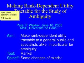
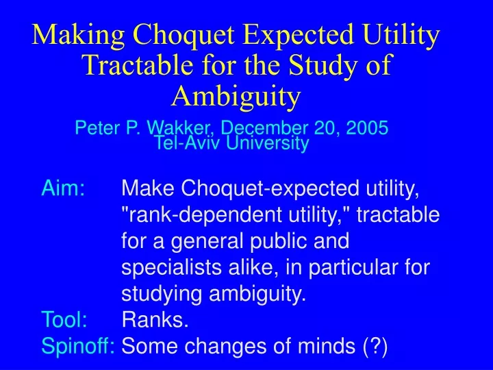
Making Choquet Expected Utility Tractable for the Study of Ambiguity. Peter P. Wakker, December 20, 2005 Tel-Aviv University. Aim: Make Choquet-expected utility, "rank-dependent utility," tractable for a general public and specialists alike, in particular for studying ambiguity. Tool: Ranks.

E N D
Making Choquet Expected Utility Tractable for the Study of Ambiguity Peter P. Wakker, December 20, 2005Tel-Aviv University Aim: Make Choquet-expected utility, "rank-dependent utility," tractable for a general public and specialists alike, in particular for studying ambiguity. Tool:Ranks. Spinoff: Some changes of minds (?)
(p1:x1,…,pn:xn) = p1 p1 x1 x1 . . . . . . . . . . . . is prospect yielding $xj with probability pj, j=1,…,n. xn xn pn pn Expectedutility: p1U(x1 ) + ... + pnU(xn) 2 • Expected Utility for Risk
3 moderately- p1 p1 q2 p2 y2 x2 . . . . . . . . . . . . p1 p1 xn ym q2 p2 pn qm y2 x2 . . . . . . . . . . . . xn ym pn qm go to p. 28, where RDU = EU for risk next p. rank- Well-known implication: Independence from common consequence ("sure-thing principle"): rank- r r r r
w w .89 .89 0 0 .10 .10 .01 .01 0 1M b b .10 .10 5M 1M > < .10 .10 .89 .89 EU 1M 1M w w .01 .01 0 1M b b .10 .10 5M 1M go to p. 27, where RDU EU for risk next p. Well-known violation of expected utility:Allais paradox. M: million $ 4 OK for RDU, with "pessimism" or "inverse-S." Is the certainty effect.
5 Other well-known violation of expected utility, for unknown probabilities: Ellsberg paradox. Known urn: 100 bals, 50 red, 50 black. Unknown urn: 100 ball, ? red, 100–? black. Common preferences: (Redknown: $100)(Redunknown: $100) & (Blackknown: $100) (Blackunknown: $100). Violate expected utility.
6 Question 1 to audience: From what can we best infer that people deviate from expected utility for risk (given probs)? a.Nash equilibria. b.Allais paradox. c.Ellsberg paradox.
7 Question 2 to audience: From what can we best infer that people deviate from expected utility for uncertainty (unknown probabilities)? a.Nash equilibria. b.Allais paradox. c.Ellsberg paradox.
8 Question 3 to audience: Assume rank-dependent utility for unknown probabilities ("Choquet Expected utility"). From what can we best infer that nonadditive measures are convex (= superadditive, "uncertainty-averse," "pessimistic")? a.Nash equilibria. b.Allais paradox. c.Ellsberg paradox.
9 After this lecture: Answer to Question 1 ("nonEU for risk") is: Allais paradox. Answer to Question 3 ("capacities convex in rank-dependent utility") is: Allais paradox! Answer to Question 2 ("nonEU for uncertainty") is: both Allais and Ellsberg paradox. P.s.: I do think that the Ellsberg paradox has more content than the Allais paradox. Explained later.
10 Related change of mind: The inequality Decision under risk Decision under uncertainty in the strict sense of [ Decision under risk Decision under uncertainty = ] is incorrect! Decision under risk Decision under uncertainty. That's how it is!
11 Idea that Allais paradox speak only to risk, and not to uncertainty, does not even make sense to me!
12 Outline of lecture: Expected Utility for Risk (almost done). Expected Utility for Uncertainty. Rank-Dependent Utility for Risk, Defined through Ranks. Where Rank-Dependent Utility Differs from Expected Utility for Risk. Where Rank-Dependent Utility Agrees with Expected Utility for Risk, and some properties. Rank-Dependent Utility for Uncertainty, Defined through Ranks. Where Rank-Dependent Utility Differs from Expected Utility for Uncertainty as it Did for Risk. Where Rank-Dependent Utility Agrees with Expected Utility for Uncertainty. Where Rank-Dependent Utility Differs from Expec-ted Utility for Uncertainty Differently than for Risk. Applications of Ranks.
13 In preparation for rank-dependence and decision under uncertainty, remember: In (p1:x1,…,pn:xn), we have the liberty to number outcomes/probs such that x1... xn.
14 2. Expected Utility for Uncertainty Wrong start for DUU: Let S = {s1,…,sn} denote a finite state space. x : S is an act, also denoted as an n-tuple x = (x1,…,xn). Is didactical mistake for rank-dependence! Why wrong? Later, for rank-dependence, ranking of outcomes will be crucial. Should use numbering of xj for that purpose; as under risk! Should not have committed to a numbering of outcomes for other reasons. So, start again:
15 S: state space, or universal event (finite or infinite). Act is function x : S with finite range. x = (E1:x1, …, En:xn): yields xj for all sEj, with: x1,…,xn are outcomes, E1, …, En are events partitioning S. No commitment to a numbering of outcomes! As for risk. This is an important notational point for rank-dependence (that model will come later). P.s.: If E1,…,En understood, we may write (x1, …,xn).
E1 E1 x1 x1 . . . . . . . . . . . . (E1:x1,…,En:xn) = xn xn En En Subjective Expected utility: (E1)U(x1 ) + ... + (E1)U(xn) 16 U: subjective index of utility. : subjective probability.
next p. next p. 17 Notation:Ex is (x with outcomes on Ereplaced by ): R and ranking position of E is R 10E1x = (E1:10,E2:x2,.., En:xn); Enx = (E1:x1,.., En-1:xn-1, En:); etc. Monotonicity: Ex Ex;
rank- go to p.42, RDU=EU next p. 18 Well-known implication: sure-thing principle: ExE y R R ExE y R R
w w L L 0 0 H H M M 0 25K (77%) b b H H 25K 75K > < H H L SEU L 25K 25K w w M M 25K (66%) 0 b b H H 25K 75K go to p.36, RDUEU next p. Almost-unknown implication 19 (Not-so-well-known) violation (MacCrimmon & Larsson '79; here Tversky & Kahneman '92). Within-subjects expt, 156 money managers. d:DJtomorrw–DJtoday.L:d<30 ;M:30d35;H:d>35; K: $1000. OK for RDU: pes-simism / inverse-S. Certainty-effect & Allais hold for uncertainty in general, not only for risk!
go to p. with ut.curv, if treated. 20 3. Rank-Dependent Utility for Risk, Defined through Ranks Empirical findings: nonlinear treatment of probabilities. Hence RDU. Two insights needed for getting the theory: Insight 1. Deviations from expected value: also caused by nonlinear perception / processing of probability, through w(p). Insight 2. Turn this into decision theory through rank-dependence.
? Rank-dependent utility of p1 x1 . . . . . . xn pn 21 • First rank-order x1>…> xn. • Decision weight of xj will depend on: • pj; • pj–1 + … + p1, the probability of receiving something better. The latter will be called a rank. • I will recommend using ranks instead of comonotonicity …
? So, rank-dependent utility of p1 x1 . . . . . . xn pn 22 First rank-order x1>…> xn. Then rank-dependent utility is 1U(x1 ) + … + nU(xn) where j = w(pj + pj–1 + …+ p1) – w(pj–1 + …+ p1). The decision weight j depends on pj and on pj–1 + …+ p1: pj–1 + …+ p1 is the rank of pj,xj, i.e. the probability of receiving something better.
23 Ranks and ranked probabilities (formalized hereafter) are proposed as central concepts in this lecture. Were introduced by Abdellaoui & Wakker (2005). With them, rank-dependent life will be easier than it was ever before!
24 In general, pairs pr, also denoted p\r, with p+r 1 are called ranked probabilities. r is the rank of p. (pr) = w(p+r) – w(r) is the decision weight of pr.
Again, rank-dependent utility of p1 x1 . . . . . . xn pn 25 with rank-ordering x1… xn: (p1r1)U(x1) + … + (pnrn)U(xn) with rj = pj–1 + …+ p1 (so r1 = 0). The smaller the rank r in pr, the better the outcome. The best rank, 0, is also denoted b, as in pb=p0. The worst rank for p, 1–p, is also denoted w, as in pw = p1–p.
26 There is a duality: For today: never mind. Rank = goodness-rank (probability of receiving an outcome ranked better). The, dual, badness-rank (probability of receving an outcome ranked worst) is sometimes more natural.
go to p. 4, with Allais 27 4. Where Rank-Dependent Utility Differs from Expected Utility for Risk Allais paradox explained by rank dependence. Now the expression "rank dependence" can be taken literally!
go to p. 3, with risk-s.th.pr 28 5. Where Rank-Dependent Utility Agrees with Expected Utility for Risk, and some Properties Sure-thing principle of EU goes through completely for RDU if we replace probability by ranked probability. Some properties, suggested by Allais paradox, follow now (more to come later). Now see Fig. of w-shaped.doc
29 w convex (pessimism): r < r´ w(p+r) – w(r) w(p+r´) – w(r´) Equivalent to: (pr) increasing in r. Remember: big rank is bad outcome. "Decision weight is increasing in rank." w concave (optimism) is similar. 2 more pessimistic than 1, i.e. w2 more convex than w1: r < r´, 1(pr) = 1(qr´) 2(pr) 2(qr´)
1 w 0 1 p 0 insensitivity-region 30 Inverse-S: How define formally? Specify b, then require concavity below, convexity above? We prefer an alternative formalization. • Specify insensitivity region in the middle. 2. Specify through inequalities that marginal w is smaller there than in extreme regions. 3. Avoid comparisons between two extreme regions (by restricting domains of inequalities).
1 w (pw) (pr) (pb) 1 bb bw p worst-rank region best-rank region insensitivity-region best-rank overweighting worst-rank overweighting 31 Inverse-S, or likelihood insensitivity, holds on region [bb,bw], if (i) and (ii) below hold. In insensitivity region, marginal w smaller than in extreme regions. p r r+p 1–p (pb) (pr) on* [0,bw] (r+p bw) (ii) (pw) (pr) on* [bb,1] (r bb). *: restricting domains to avoid comparisons between two extreme regions.
32 6. Rank-Dependent Utility for Uncertainty, Defined through Ranks x = (E1:x1, …, En:xn) was act, with Ej's partitioning S. Rank-dependent utility for uncertainty: (also called Choquet expected utility) W is capacity, i.e. (i) W() = 0;(ii) W(S) = 1 for the universal event S;(iii) If A B then W(A) W(B) (monotonicity with respect to set inclusion).
33 ER, with ER = , is ranked event, with R the rank. (ER) = W(ER) – W(R) is decision weight of ranked event. RDU of x = (E1:x1, …, En:xn), with rank-ordering x1… xn, is:jn(EjRj)U(xj) with Rj = Ej–1 … E1 (so R1 = ). Compared to SEU, ranks Rj have now been added, expressing rank-dependence.
34 The smaller the rank R in ER, the better the outcome. The best (smallest) rank, , is also denoted b, as in Eb = E. The worst (biggest) rank for E, Ec, is also denoted w, as in Ew = EEc.
35 Difficult notation in the past: S = {s1,…,sn}. For RDU(x1,…,xn), take a rank-ordering r of s1,...,sn such that xr1 ... xrn. For each state srj, prj = W(srj,…, sr1) – W(srj-1,…, sr1) RDU = pr1U(xr1) + … + prnU(xrn) Due to -notation, difficult to handle. (2) = 5: Is state s2 fifth-best, or is state s5 second-best? I can never remember!
go to p. 19, Allais for uncertainty 36 7. Where Rank-Dependent Utility Differs from Expected Utility for Uncertainty as It Did for Risk Convexity of W follows from Allais paradox! Easily expressable in terms of ranks: (ER) increasing in R.
go to p. on TO measuement etc. if presented 37 8. Where Rank-Dependent Utility Agrees with Expected Utility for Uncertainty The whole measurement of utility, and preference characterization, of RDU for uncertainty is just the same as SEU, if we simply use ranked events instead of events!
38 9. Where Rank-Dependent Utility Differs from Expected Utility for Uncertainty Differently than It Did for Risk Allais: deviations from EU. Pessimism/convexity of w/W, or insensitivity/inverse-S. For risk and uncertainty alike. Deviations from EU in an absolute sense. Ellsberg: more deviations from EU for uncertainty than for risk. More pessimism/etc. for uncertainty than for risk. Deviations from EU in an relative sense. Deviations from EU: byproduct.
39 Historical coincidence: Schmeidler (1989) assumed EU for risk, i.e. linear w. Then: more pessimism/convexity for uncertainty than for risk (based on Ellsberg), pessimism/convexity for uncertainty. Voilà source of numerous misunderstandings.
40 Big idea to infer of Ellsberg is not, I think, ambiguity aversion. Big idea to infer from Ellsberg is, I think, within-person between-source comparisons. Not possible for risk, because risk is only one source. Typical of uncertainty, where there are many sources. Uncertainty is a rich domain, with no patterns to be expected to hold in great generality. In this rich domain, many phenomena are present and are yet to be discovered.
41 10. Applications of Ranks General technique for revealing orderings (AR) (BR´) from preferences: Abdellaoui & Wakker (2005). Thus, preference foundations can be given for everything written hereafter.
42 What is null event? Important for updating, equilibria, etc. E is null if W(E) = 0? E is null if W(Ec) = 1? E is null if (H:, E:, L:) ~ (H:, E:, L:)? For some , H …? Or for all , H …? ? We: Wrong question! Better refer to ranked events! (Eb) = 0. (Ew) = 0. (EH) = 0. Plausible condition is null-invariance: independence of nullness from rank.
(1) Insensitivity-region is [Bb,Bw]. on event-interval [,Bw] (ERBw) on event-interval [Bb,S] (RBb) (Eb) (ER) (Ew) (ER) (2) (3) 43 W convex: increases in rank. W concave: decreases in rank. W symmetric: (Eb) = (Ew). Inverse-S: (1) Specify (“event-”)insensitivity-region; (2) Specify through inequalities that marginal W is smaller there than in extreme regions. (3) Avoid comparisons between two extreme regions (by restricting domains of inequalities).
44 Theorem. 2 is more ambiguity averse than 1 in sense that W2 is more convex than W1 iff 1(BR´) = 1(AR) with R´ R 2(BR´) 2(AR).
45 Theorem. Probabilistic sophistication holds [(AR) (BR) (AR´) (BR´)]. In words: ordering of likelihoods is independent of rank.
W(A) . W(B) W(ABc) – W(Bc) W(A) . . 1 – W(Bc) W(A) + 1 – W((B\A)c) (Ab) (ABc) (Ab) (Ab) + ((B\A)w) (Bw) (Bb) 46 Updating on A given B, with A B. What is W(A) if B is observed? Gilboa (1989a,b): Dempster & Shafer: Jaffray, Denneberg: Gilboa & Schmeidler (1993): depends on optimism / pessimism. Ranks formalize this. Cohen,Gilboa,Jaffray,&Schmeidler (2000): lowest one did best.
47 Conclusion: With ranks and ranked probabilities or events, rank-dependent-utility/Choquet-expected-utility becomes considerably more tractable.
48 The end!
0.10 0.30 0.50 0.90 0.70 $100 $100 $100 $100 $100 ~ ~ ~ ~ ~ $25 $81 $49 $9 $1 0 0 0 0 0 0.70 0.50 0.10 0.30 0.90 (b) (c) (d) (a) (e) 1 $100 p $ (e) (e) 0.7 $70 (d) (d) (c) (c) (b) 0.3 $30 (b) (a) (a) 0 $0 $0 $100 $30 $70 0 1 0.3 0.7 p $ go to p.27,RDU next p. 49 Assume following data deviating from expected value U(100) = 1, U(0) = 0 U(1) = 0.10U(100) + 0.90U(0) = 0.10. EU: EU: U(x) = pU(100) = p. Here is graph of U(x): EU: U(9) = 0.30U(100) = 0.30. Psychology: x = w(p)100 Here is graph of w(p): Psychology: 1 = w(.10)100