Download
1 / 21
210 likes | 298 Views
Chesapeake Bay Lagrangian Floats Analysis. Motivation. Lagrangian float has its advantage in describing waters from different origins. We follow definition of M as along trajectory speed of floats.

E N D
Motivation • Lagrangian float has its advantage in describing waters from different origins. We follow definition of M as along trajectory speed of floats. • M function itself can be calculated in 3 dimensions but is usually applied to 2 dimensional ocean processes. On different time scales, flows are 3D (upwelling etc) and M need to be analyzed in 3D. • Chesapeake Bay is a partially mixed estuary, two layer flows are typical flow structure near the Bay Mouth. Out flow Plumes on the surface are highly non-linear rapidly responding to wind stress. • Hypothesis: 3D M function can be used to track the fresh(er) water from the bay, to detect the interface between the two-layer flow, to distinct the sharp boundary of plume and to evaluate transport exchange between plume and ambient water • Expected Problems: Mixing can quickly blur the M function, periodical tidal flows and wind modulation makes the flow quite complicated.
Study Methods • Simulate the Chesapeake Bay Estuary Circulation including outflow plume region using a regional ocean modeling system. • Calculate M function in 3D simulated velocity fields and analyze M representing different ocean processes.
Model Setup • Regional Ocean Modeling System (ROMS) • Oregon State University Tide Prediction System • USGS river discharge • North American Regional Analysis • ETOPO 1 minutes resolution • Climatology of open boundary Temperature and Salinity from WOA ¼ degree (no nesting)
Model Forcing USGS river discharge NARR Wind Vectors Near Bay Mouth OTPS M2 Tidal current ellipse (only imposed along open boundary)
M function calculation • M function: • Forward and Backward offline Calculation respectively • Fourth-order Milne predictor and fourth-order Hamming corrector • Time Step: 2 minutes (versus 1-hour) • Land/sea boundary: free slip
M sensitive to time step 2 Min 1 Hour Discussion: It looks this is related to the land/sea boundary, if a non-slip boundary condition is set, the difference might be much smaller. We use a free-slip boundary condition. A test need to be added. If there is no land/sea boundary, the time step of 1 hour (or more) seems OK even tidal flow presents. Difference: 2min-1hour
M sensitive to time τ Simulated Barotropic M2 Tidal Ellipse τ=1day τ=2day • As τ is set to 3 or 4 days, the M structure is richer, but it is more difficult to interpret. • Tidal flow in the mid bay is strong, large M simply corresponds to several strong tidal cycle along the bay. • Online and offline version is consistent when time step is the same. τ=3day τ=4day
Mid Bay (τ=4 days) M Forward Backward Online Foward Dominated by tidal flow, other subtidal flow feature are difficult to detect. But patch of M is shifted by winds (another wind figure is needed). http://zilla.umd.edu/~bzhang/CBFS/Floats/Report/2minutes/Surface/10.html
Summary • Offline M function agrees with online calculation (forward only) . • M in the mid-bay is dominated by tides (modulated by winds). • With larger τ, M structure is richer due to floats undergoing more tidal cycle. • We are also interested in the two layer flow and plume near the bay mouth. Especially on the downwelling wind favorable condition when a plume can be easily confined on the coast and detectable in the model.
Monthly Mean Subtidal Flow A simple experiment to use M in a constant flow structure, typical two layer flow
M of the Mean Flow along Transect M is different from Eulerian flow, implying upwelling favorable wind dominates during this month. Outflow tends to northeast and hence brings particles there more rapidly. Lower values in M indicates possible interface of the two-layer flow. Vertical velocity on the interface does not necessily be zero (mixing)
M with full time velocity (02/08 6:00, τ=2days) South North The red patch represents most of outgoing flow. Inflow lies against bottom. Dashed lines represent backward float path. More patterns will be looked at different time.
Plume in a Eulerian Salinity field We particularly look at the plume at a downwelling favorable wind condition. Two layer flow and sharp plume boundary (both in horizontal and vertical direction) are expected.
Surface Plume in Lagrangian View (M) =1 days =2 days =4 days =3 days Clear, sharp gradient at all times, but larger τ has more feature. M
Float Path with Time Several small scale cyclone(anticyclone) eddies can be observed in the model during one tidal cycle, these eddies interact with the plume. Looking further at the mixing and transport. Note: Surface water will stay on the surface without considering vertical mixing and momentum sink.
Vertical Transition (=2days) 02 01 03 04 05 07 06 08 09 10
Two Layer Flows and M function This is very different from the mean flow situation, where large M is confined near the coast (note location and integration time is different too). This provides clear measurements to the plume instead from mean velocity or instant velocity fields.
M animation along sect 3 (τ=4days) http://zilla.umd.edu/~bzhang/CBFS/Floats/Plume/sect/sect03/