Goodfellow: Chap 6 Deep Feedforward Networks

1. Goodfellow: Chap 6Deep Feedforward Networks Dr. Charles Tappert The information here, although greatly condensed, comes almost entirely from the chapter content.

2. Introduction to Part II • This part summarizes the state of modern deep learning for solving practical applications • Powerful framework for supervised learning • Describes core parametric function approximation • Part II important for implementing applications • Technologies already used heavily in industry • Less developed aspects appear in Part III

3. Chapter 6 Sections • Introduction • 1 Example: Learning XOR • 2 Gradient-Based Learning • 2.1 Cost Functions • 2.2 Output Units • 3 Hidden Units • 3.1 Rectified Linear Units and Their Generalizations • 3.2 Logistic Sigmoid and Hyperbolic Tangent • 3.3 Other Hidden Units • 4 Architecture Design • 4.1 Universal Approximation Properties and Depth • 4.2 Other Architectural Considerations • 5 Back-Propagation and Other Differentiation Algorithms

4. Chapter 6 Sections (cont) • 5 Back-Propagation and Other Differentiation Algorithms • 5.1 Computational Graphs • 5.2 Chain Rule of Calculus • 5.3 Recursively Applying the Chain Rule to Obtain Backprop • 5.4 Back-Propagation Computation in Fully-Connected MLP • 5.5 Symbol-to-Symbol Derivatives • 5.6 General Back-Propagation • 5.7 Example: Back-Propagation for MLP Training • 5.8 Complications • 5.9 Differentiation outside the Deep Learning Community • 6 Historical Notes

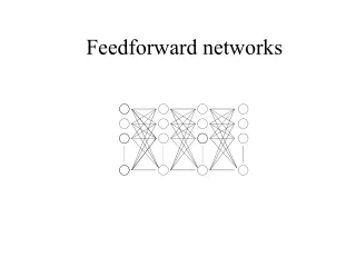
5. Introduction • Deep Feedforward Networks • = feedforward neural networks = MLP • The quintessential deep learning models • Feedforward means forward flow from x to y • Networks with feedback called recurrent networks • Network means composed of sequence of functions • Model has a directed acyclic graph • Chain structure – first layer, second layer, etc. • Length of chain is the depth of the model • Neural because inspired by neuroscience

6. Introduction (cont) • The deep learning strategy is to learn the nonlinear input-to-output mapping • The mapping function is parameterized and an optimization algorithm finds the parameters that corresponds to a good representation • The human designer only needs to find the right general function family and not the precise right function

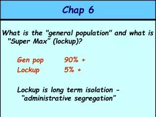
7. 1 Example: Learning XOR • The challenge in this simple example is to fit the training set – no concern for generalization • We treat this as a regression problem using the mean squared error (MSE) loss function • We find that a linear model cannot represent the XOR function

8. SolvingXOR Originalxspace Learnedhspace 1 1 h2 x2 0 0 0 1 0 1 h1 2 x1 Figure6.1 (Goodfellow2016)

9. 1 Example: Learning XOR • To solve this problem, we use a model with a different feature space • Specifically, we use a simple feedforward network with one hidden layer having two units • To create the required nonlinearity, we use an activation function, the default in modern neural networks the rectified linear unit (ReLU)

10. NetworkDiagrams y y h1 h2 h W x1 x2 Figure6.2 (Goodfellow2016)

11. RectifiedLinearActivation g(z)=max{0,z} 0 0 z Figure6.3 (Goodfellow2016)

12. 1 Example: Learning XOR

13. 1 Example: Learning XOR

14. SolvingXOR Originalxspace Learnedhspace 1 1 h2 x2 0 0 0 1 0 1 h1 2 x1 Figure6.1 (Goodfellow2016)

15. Duda, Chap 6 (other book) Pattern Classification, Chapter 6

16. 2 Gradient-Based Learning • Designing and training a neural network is not much different from training other machine learning models with gradient descent • The largest difference between the linear models we have seen so far and neural networks is that the nonlinearity of a neural network causes most interesting loss functions to become non-convex

17. 2 Gradient-Based Learning • Neural networks are usually trained by using iterative, gradient-based optimizers that drive the cost function to a low value • However, for non-convex loss functions, there is no convergence guarantee

18. 2.1 Cost Functions • The choice of a cost function is important • Maximum likelihood • Functional (a conditional statistic), such as “mean absolute error”

19. 2.2 Output Units • The choice of a cost function is tightly coupled with the choice of output unit • Linear units for Gaussian output distributions • Sigmoid units for Bernoulli output distributions • Softmax units for Multinoulli output distributions • Others

20. 3 Hidden Units • Choosing the type of hidden unit • Rectified linear units (ReLU) – the default choice • Not differentiable at z = 0 • Okay, because training will not go to gradient of 0 • Logistic sigmoid and hyperbolic tangent • Others

21. 4 Architecture Design • Overall structure of the network • Number of layers, number of units per layer, etc. • Layers arranged in a chain structure • Each layer being a function of the preceding layer • Ideal architecture for a task must be found via experiment, guided by validation set error

22. 4.1 Universal Approximation Properties and Depth • Universal approximation theorem • Regardless of the function we are trying to learn, we know that a large MLP can represent it • In fact, a single hidden layer can represent any function • However, we are not guaranteed that the training algorithm will be able to learn that function • Learning can fail for two reasons • Training algorithm may not find solution parameters • Training algorithm might choose the wrong function due to overfitting

23. 4.2 Other Architectural Considerations • Many architectures developed for specific tasks • Many ways to connect a pair of layers • Fully connected • Fewer connections, like convolutional networks • Deeper networks tend to generalize better

24. Better Generalization with Greater Depth 96.5 96.0 95.5 95.0 94.5 94.0 93.5 93.0 92.5 92.0 Testaccuracy(percent) 3 4 5 6 7 8 9 10 11 Layers (Goodfellow2016)

25. Large,ShallowModelsOverfitMore 97 3,convolutional 3,fullyconnected 11,convolutional Testaccuracy(percent) 96 95 Layers 94 93 92 91 0.0 0.2 0.4 0.6 Numberofparameters 0.8 1.0 ⇥108 Shallow models tend to overfit around 20 million parameters, deep ones benefit with 60 million (Goodfellow2016)

26. 5 Back-Propagation and Other Differentiation Algorithms • When we accept an input x and produce an output y, information flows forward in network • During training, the back-propagation algorithm allows information from the cost to flow backward through the network in order to compute the gradient • The gradient is then used to perform training, usually through stochastic gradient descent

27. 5.1 Computational Graphs • Useful to have a computational graph language • Operations are used to formalize the graphs

28. ComputationGraphs yˆ z u(1) u(2) + dot y X b X W (a) (b) u(2) u(3) H relu sum x U(1) U(2) u(1) yˆ + sqr dot matmul X W b X l W (c) (d) (Goodfellow2016)

29. 5.2-10 Chain Rule and Partial Derivatives

30. Symbol-to-Symbol Differentiation z z Figure6.10 f f f' dz dy y y f f f' x dy dz x x dx dx f f x f' dx dz w w dw dw (Goodfellow2016)

31. 6 Historical Notes • Leibniz (17th century) – derivative chain rule • Rosenblatt (late 1950s) – Perceptron learning • Minsky & Papert (1969) – critique of Perceptrons caused 15-year “AI winter” • Rumelhart, et al. (1986) – first successful experiments with back-propagation • Revived neural network research, peaked early 1990s • 2006 – began modern deep learning era