Download
1 / 59
730 likes | 1.44k Views
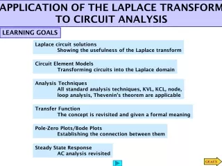
THE LAPLACE TRANSFORM IN CIRCUIT ANALYSIS. +. +. R. R. i. I. v. V. A Resistor in the s Domain. v=Ri (Ohm’s Law). V(s)=RI(s. I 0 s. An Inductor in the s Domain. Initial current of I 0. V(s)=L[sI(s)-i(0 - )]=sLI(s)-LI 0. +. L. i. v. I. +. sL. I. +. V. sL. V. LI 0. +.

E N D
+ + R R i I v V A Resistor in the s Domain v=Ri (Ohm’s Law). V(s)=RI(s
I0 s An Inductor in the s Domain Initial current of I0 V(s)=L[sI(s)-i(0-)]=sLI(s)-LI0 + L i v I + sL I + V sL V LI0 +
+ i v C A Capacitor in the s Domain Initially charged to V0 volts. I + 1/sC I + 1/sC CV0 V V + V0/s
t=0 + + C i v V0 The Natural Response of an RC Circuit + 1/sC I R R V + V0/s
Transient Response of a Parallel RLC Circuit Replacing the dc current source with a sinusoidal current source
Thevenin’s Theorem Use the Thevenin’s theorem to find vc(t)
MUTUAL INDUCTANCE EXAMPLE i2(t)=?
MUTUAL INDUCTANCE EXAMPLE Using the T-equivalent of the inductors, and s-domain equivalent gives the following circuit
THE TRANSFER FUNCTION The transfer function is defined as the ratio of the Laplace transform of the output to the Laplace transform of the input when all the initial conditions are zero. Y(s) is the Laplace transform of the output, X(s) is the Laplace transform of the input.
EXAMPLE Find the transfer function V0/Vg and determinethe poles and zeros of H(s).
Assume that vg(t)=50tu(t). Find v0(t). Identify the transient and steady-state components of v0(t).
The transient component is generated by the poles of the transfer function and it is: The steady-state components are generated by the poles of the driving function (input):
Time Invariant Systems If the input delayed by a seconds, then Therefore, delaying the input by a seconds simply delays the response function by a seconds. A circuit that exhibits this characteristic is said to be time invariant.
Impulse Response If a unit impulse source drives the circuit, the response of the circuit equals the inverse transform of the transfer function. Note that this is also the natural response of the circuit because the application of an impulsive source is equivalent to instantaneously storing energy in the circuit.
x(t) x(t) y(t) y(t) N N CONVOLUTION INTEGRAL x(t) y(t) t a b t a b Circuit N is linear with no initial stored energy. If we know the form of x(t), then how is y(t) described? To answer this question, we need to know something about N. Suppose we know the impulse response of the system. (1) t t
Instead of applying the unit impulse at t=0, let us suppose that it is applied at t=λ. The only change in the output is a time delay. N Next, suppose that the unit impulse has some strength other than unity. Let the strength be equal to the value of x(t) when t= λ. Since the circuit is linear, the response should be multiplied by the same constant x(λ) N
Now let us sum this latest input over all possible values of λ and use the result as a forcing function for N. From the linearity, the response is the sum of the responses resulting from the use of all possible values of λ N From the sifting property of the unit impulse, we see that the input is simply x(t) N X(t)
Our question is now answered. When x(t) is known, and h(t), the unit impulse response of N is known, the response is expressed by This important relation is known as the convolution integral. It is often abbreviated by means of Where the asterisk is read “convolved with”. If we let z=t-λ, then dλ=-dz, and the expression for y(t) becomes
Convolution and Realizable Systems For a physically realizable system, the response of the system cannot begin before the forcing function is applied. Since h(t) is the response of the system when the unit impulse is applied at t=0, h(t) cannot exist for t<0. It follows that, in the second integral, the integrand is zero when z<0; in the first integral, the integrand is zero when (t-z) is negative, or when z>t. Therefore, for realizable systems the convolution integral becomes
EXAMPLE x(t) y(t) h(t) 1 t
Since h(z) does not exist prior to t=0 and vi(t-z) does not exist for z>t, product of these functions has nonzero values only in the interval of 0<z<t for the case shown where t<1. When t>1, the nonzero values for the product are obtained in the interval (t-1)<z<t.
EXAMPLE Apply a unit-step function, x(t)=u(t), as the input to a system whose impulse response is h(t) and determine the corresponding output y(t)=x(t)*h(t).
When t<0, there is no overlap and y(t)=0 for t<0 For 0<t<1, the curves overlap from z=0 to z=t and product is 1. Thus, When 1<t<2, h(t-z) has slid far enough to the right to bring under the step function that part of the negative square extending from 0 to z=t-1. Thus,
Finally, when t>2, h(t-z) has slid far enough to the right so that it lies entirely to the right of z=0
Convolution and the Laplace Transform Let F1(s) and F2(s) be the Laplace transforms of f1(t) and f2(t), respectively. Now, consider the laplace transform of f1(t)*f2(t), Since we are dealing with the time functions that do not exist prior to t=0-, the lower limit can be changed to 0-
f1(λ) does not depend on t, and it can be moved outside the inner integral
STEADY-STATE SINUSOIDAL RESPONSE If the input of a circuit is a sinusoidal function
The partial fraction expansion of Y(s) is If the poles of H(s) lie in the left half of the s plane, the corresponding time-domain terms approach zero as t increases and they do not contribute to the steady-state response. Thus only the first two terms determine the steady-state response.