Download
1 / 38
380 likes | 503 Views
COST-722. COSMO User’s Seminar. Langen, March 2008. Intercomparison of European Fog Forecast Models. M.Masbou 1,2 , A. Bott 1 , M. D. Müller 3 , N. W.Nielsen 4 , C. Petersen 4 , H. Seidl 5 , A. Kann 5 , J. Cermak 6 , H. Petithomme 7 & W. K. Adam 8.

E N D
COST-722 COSMO User’s Seminar Langen, March 2008 Intercomparison of European Fog Forecast Models M.Masbou1,2, A. Bott1, M. D. Müller3, N. W.Nielsen4, C. Petersen4, H. Seidl5, A. Kann5, J. Cermak6, H. Petithomme7 & W. K. Adam8 1 Meteorological Institute, University of Bonn, Germany, mmasbou@uni-bonn.de 2 Laboratoire de Météorologie physique, University Blaise Pascal, Clermont-Ferrand, France 3 Institute of Meteorology, Climatology & Remote Sensing, University of Basel, Switzerland 4 Danish Meteorlogical Institute, Copenhagen, Denmark 5 Central Institute for Meteorology and Geodynamics, Vienna, Austria 6 Laboratory for Climatology & Remote Sensing, University of Marburg, Germany 7 Meteo France, Toulouse, France 8 Meteorological Observatory Lindenberg, DWD, Germany
Fog Formation 1D 3D • Cooling • Moistening • Turbulent Mixing • Reach saturation Radiation fog Advection fog (1D) 3D 3D Upslope fog Valley fog Precipitation fog
Fog: A visibility reduction 1.4km 1km 0.5 km 100 m 50 m
COST 722 Project Development of advanced methods for short-range forecasts of fog, visibility and low clouds Working Group I: Initial Data • Improved calibration and analysis of satellite data • Recommendation of measurement equipments • Exchange of knowledge and methods Working Group II: Numerical Models • Developement of numerical for fog and low clouds • Improved understanding of physical processes during fog events Working Group III: Statistical Methods • Powerful and highly sophisticated statisitcal methods • Improved expertise on statistical methods • Basis for the preparation of training material
Comparison Campaign on the Lindenberg Area September – December 2005 Phase 1: Statistics Each Participant produce 4 month fog forecast and quantify statistically his fog forecast quality (FAR, HR, ETS) Phase 2: Fine Comparison for chosen fog/no fog events Episode 1: fog formation with mid cloud cover September, 27th 2005: 01-05 UTC Episode 2: fog formation with without cloud cover October, 6th 2005: 07-09 UTC October, 7th 2005: 06-08 UTC Episode 3: fog formation with 8/8 cloud cover December, 6th 2005: 18-00 UTC December, 7th 2005: 00-23 UTC
Lindenberg Area Observatory of DWD supplies: • Visibility 2m • Cloud cover • Radiative fluxes (SW, LW, Latent and Sensible) • 10m-Mast: T, RH, Wind • 100m-Mast: T, RH, Wind • Radiosounding (00, 06, 12 and 18 UTC) • Soil temperature • Soil moisture
Participants Statistical Model: MOS-ARPEGE France: H. Petithomme MOS statistics using linear discriminant analysis Uses model output of the hydrostatic global model ARPEGE Predictand: visibility with different thresholds Predictor: pressure at the ground, cloud cover, 10m wind speed, RH2m, T2m
Operational models Austria: H. Seidl and A. Kann Model name: ALADIN-AUSTRIA Resolution: 9.6 km horizontal, 45 vertical layers Model domain: Europe Boundary values: global model ARPEGE Dynamics: Hydrostatic Turbulence: Louis scheme Visibility:Post-processing in case of T-inversion gradient RH and T Denmark: C. Petersen and N.W. Nielsen Model name: DMI-HIRLAM Resolution: 16 km horizontal, 40 vertical layers Model domain: Europe Boundary values: ECMWF analyses and forecasts Dynamics: Hydrostatic Turbulence: prognostic TKE Visibility:MOS approach depending on ground measurements and model forecasts
Non-operational models Germany: M. Masbou and A. Bott Model name: LM-PAFOG (COSMO-FOG) Resolution: 2.8 km horizontal, 40 vertical layers, Δzmin=4m Model domain: 280 x 280 km limited area Boundary values: COSMO-EU Dynamics: Nonhydrostatic, fully compressible Turbulence: Louis scheme Visibility:diagnostic variable depending on CCN, LWC, aerosol concentration at 2m Switzerland: M.D. Müller Model name: NMM-PAFOG Resolution: 1 km horizontal, 45 vertical layers Model domain: 160 x 160 km limited area Boundary values: NMM 13 km Dynamics: Nonhydrostatic, fully compressible Turbulence: prognostic TKE Visibility: complex relation of moist forecasted parameter at 2m
Statistical Study METHOD Comparison 1 pixel of Model area with visibility 2m 5 Categories: < 350m, < 600m, < 1000m, < 1500m, < 3000m Basing on contingence table analyses PERIOD 4 months forecast (September-December 2005) MODELS Initialization: each day at 00 UTC FOG CLIMATOLOGY 35 Fog events Fog episode very rare, 4 % of studied time period
Ensemble Forecast To analyse the basic quality of the European models Ensemble forecast extracted from the 4 models Fog event probability of the ensemble Fog event probability of the i-th model Quantity of available forecasts Average out disagreements between ensemble member
Hit Rate What fraction of the observed “fog" events were correctly forecast? BLACK:LM-PAFOG RED:ENSEMBLE GREEN:HIRLAM MAGENTA:MOS-ARPEGE BLUE:ALADIN
False Alarm Rate What fraction of the observed "no-fog" events were incorrectly forecast as “fog"? BLACK:LM-PAFOG RED:ENSEMBLE GREEN:HIRLAM MAGENTA:MOS-ARPEGE BLUE:ALADIN
False Alarm Ratio What fraction of the predicted “fog" events actually did not occur (i.e., were false alarms)? BLACK:LM-PAFOG RED:ENSEMBLE GREEN:HIRLAM MAGENTA:MOS-ARPEGE BLUE:ALADIN
Equitable Threat Score How well did the forecast “fog" events correspond to the observed “fog" events? BLACK:LM-PAFOG RED:ENSEMBLE GREEN:HIRLAM MAGENTA:MOS-ARPEGE BLUE:ALADIN
Case I: Visibility 2m Date: September, 26-27 th 2005 After a rain episode bringing warm and humid air, residual cloud parcel Radiative fog
Visibility 2m: case I Legend: Vis <1000 m >1000 m Vis <3000 m VIS-2m-NMM-PAFOG-2709200503 Lindenberg
LWC 2m: case I Legend: LWC> 0.1g/kg >0.01 g/kg LWC <0.1 g/kg Lindenberg
Case I: Vertical profile at Lindenberg BLACK:OBSERVED RED:LM-PAFOG GREEN:ALADIN BLUE:HIRLAM CYAN= NMM-PAFOG
Case II: Visibility 2m Date: December, 6-7 th 2005 Stable moist layer with a tendency to light rain, full cloud cover Low stratus and Fog
Visibility 2m: case II Legend: Vis <1000 m >1000 m Vis <3000 m VIS-2m-NMM-PAFOG-2709200503 Lindenberg
LWC 2m: case II Legend: LWC> 0.1g/kg >0.01 g/kg LWC <0.1 g/kg Lindenberg
Case II: Vertical profile at Lindenberg BLACK:OBSERVED RED:LM-PAFOG GREEN:ALADIN BLUE:HIRLAM CYAN= NMM-PAFOG
CONCLUSION • 4 Models involved NO BEST MODEL • MOS-ARPEGE: statistic model • ALADIN-AUSTRIA, DMI-HIRLAM: 3D mesoscale models, ad hoc cloud water near the surface • NMM-PAFOG, LM-PAFOG : 3D high-resolution fog forecast model, complex microphysics Statistical and fine Analysis of autumn 2005´s fog events • 20 % of the fog forecast according with measurements • Initialization and Assimilation of the boundary layer determinant role for a successful fog forecast • Visibility parameterization: decisive key • Vertical diffusion usually not designed to work well near the surface
Outlooks • Adaptedturbulent scheme for high vertical resolution • Long time verification of 3D fog forecast modelconsidering spatial distribution of fog • Adjusting the visibility parameterization Thanks COST 722
Parameters in Fog Formation Important Parameters in Fog Formation Cooling of moist air by radiative flux divergence Vertical mixing of heat and moisture Vegetation Horizontal and vertical wind Heat and moisture transport in soil Advection Topographic effect Once the fog has formed Longwave radiative cooling at fog top Gravitational droplet settling Fog microphysics Shortwave radiation (Duynkerke, P.G.,1991)
What is FOG ? WMO definition “Suspension of very small, usually microscopic water droplets in the air, generally reducing the horizontal visibility at the Earth´s surface to less than 1km” Forecaster definition (Roach, W.T., 1994) “Fog occurs whenever the horizontal visibility falls below 1km. Cloud base descending to ground level is also experienced as fog.”
Case III: Visibility 2m Date: October, 6-7 th 2005 Under influence of high pressure system, no cloud cover Radiative fog
Visibility 2m: case III Legend: Vis <1000 m >1000 m Vis <3000 m VIS-2m-NMM-PAFOG-2709200503 Lindenberg
LWC 2m: case III Legend: LWC> 0.1g/kg >0.01 g/kg LWC <0.1 g/kg Lindenberg
Case III: Vertical profile at Lindenberg BLACK:OBSERVED RED:LM-PAFOG GREEN:ALADIN BLUE:HIRLAM CYAN= NMM-PAFOG