Download
1 / 47
470 likes | 568 Views
Chapter 29: Maxwell’s Equations and Electromagnetic Waves. Displacement current. Displacement Current & Maxwell’s Equations. Displacement current (cont’d). Displacement Current & Maxwell’s Equations. Displacement current (cont’d). Displacement Current & Maxwell’s Equations.

E N D
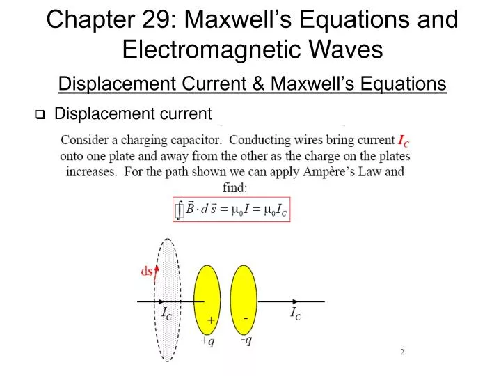
Chapter 29: Maxwell’s Equations and Electromagnetic Waves • Displacement current Displacement Current & Maxwell’s Equations
Displacement current (cont’d) Displacement Current & Maxwell’s Equations
Displacement current (cont’d) Displacement Current & Maxwell’s Equations
Displacement current (cont’d) Displacement Current & Maxwell’s Equations
Displacement current (cont’d) Displacement Current & Maxwell’s Equations
Displacement current : Example Displacement Current & Maxwell’s Equations
Maxwell’s equations: Gauss’s law Displacement Current & Maxwell’s Equations
Maxwell’s equations: Gauss’ law for magnetism Displacement Current & Maxwell’s Equations
Maxwell’s equations: Farady’s law Displacement Current & Maxwell’s Equations
Maxwell’s equations: Ampere’s law Displacement Current & Maxwell’s Equations
Maxwell’s equations Displacement Current & Maxwell’s Equations
Maxwell’s equations Gauss’s law Gauss’s law for magnetism Maxwell’s Equations and EM Waves Farady’s law Ampere’s law
Maxwell’s equations: Differential form Displacement Current & Maxwell’s Equations
Maxwell’s Equations and EM Waves • Oscillating electric dipole • First consider static electric field produced by • an electric dipole as shown in Figs. • Positive (negative) charge at the top (bottom) • Negative (positive) charge at the top (bottom) • Now then imagine these two charge are moving • up and down and exchange their position at every • half-period. Then between the two cases there is • a situation like as shown in Fig. below: What is the electric field in the blank area?
Maxwell’s Equations and EM Waves • Oscillating electric dipole (cont’d) Since we don’t assume that change propagate instantly once new position is reached the blank represents what has to happen to the fields in meantime. We learned that E field lines can’t cross and they need to be continuous except at charges. Therefore a plausible guess is as shown in the right figure.
Maxwell’s Equations and EM Waves • Oscillating electric dipole (cont’d) What actually happens to the fields based on a precise calculate is shown in Fig. Magnetic fields are also formed. When there is electric current, magnetic field is produced. If the current is in a straight wire circular magnetic field is generated. Its magnitude is inversely proportional to the distance from the current.
Maxwell’s Equations and EM Waves • Oscillating electric dipole (cont’d) What actually happens to the fields based on a precise calculate is shown in Fig.
Maxwell’s Equations and EM Waves • Oscillating electric dipole (cont’d) This is an animation of radiation of EM wave by an oscillating electric dipole as a function of time.
+ + - - - - + + Maxwell’s Equations and EM Waves • Oscillating electric dipole (cont’d) V(t)=Vocos(t) X B B • time t=/ • one half cycle later • time t=0 At a location far away from the source of the EM wave, the wave becomes plane wave.
+ + - - Maxwell’s Equations and EM Waves • Oscillating electric dipole (cont’d)
Maxwell’s Equations and EM Waves • Oscillating electric dipole (cont’d) • A qualitative summary of the observation of this example is: • The E and B fields are always at right angles to each other. • The propagation of the fields, i.e., their direction of travel away from the • oscillating dipole, is perpendicular to the direction in which the fields • point at any given position in space. • In a location far from the dipole, the electric field appears to form closed • loops which are not connected to either charge. This is, of course, always • true for any B field. Thus, far from the dipole, we find that the E and B • fields are traveling independent of the charges. They propagate away from • the dipole and spread out through space. In general it can be proved that accelerating electric charges give rise to electromagnetic waves.
Periodic waves • When particles of the medium in a wave undergo periodic • motion as the wave propagates, the wave is called periodic. l wavelength A = amplitude t=0 x=0 x Types of mechanical waves t=T/4 t=T period
Wave function • The wave function describes the displacement of particles • or change of E/B field in a wave as a function of time and • their position: • A sinusoidal wave is described by the wave function: sinusoidal wave moving in +x direction Mathematical description of a wave velocity of wave, NOT of particles of the medium angular frequency period wavelength sinusoidal wave moving in -x direction v->-v phase velocity
Wave function (cont’d) l wavelength t=0 x x=0 Mathematical description of a wave (cont’d) t=T/4 t=T period
Wave number and phase velocity wave number: phase Mathematical description of a wave (cont’d) The speed of wave is the speed with which we have to move along a point of a given phase. So for a fixed phase, phase velocity
Particle velocity and acceleration in a sinusoidal wave velocity Mathematical description of a wave (cont’d) acceleration Also wave eq.
y x z • Plane EM wave Plane EM Waves and the Speed of Light
Semi-qualitative description of plane EM wave Consider a sheet perpendicular to the screen with current running toward you. Visualize the sheet as many equal parallel fine wires uniformly spaced close together. Plane EM Waves and the Speed of Light The magnetic field from this current can be found using Ampere’s law applied to a rectangle so that the rectangle’s top and bottom are equidistance from the current sheet in opposite direction.
Semi-qualitative description of plane EM wave (cont’d) B d Plane EM Waves and the Speed of Light B L
Semi-qualitative description of plane EM wave (cont’d) Applying Ampere’s law to the rectangular contour, there are contributions only from the top and bottom because the contributions from the sides are zero. The contribution from the top and bottom is 2BL. Denoting the current density on the sheet is I A/m, the total current enclosed by the rectangle is IL. Plane EM Waves and the Speed of Light Note that the B field strength is independent of the distance d from the sheet. Now consider how the magnetic field develops if the current in the sheet is suddenly switched on at time t=0. Here we assume that sufficiently close to the sheet the magnetic field pattern found using Ampere’s law is rather rapidly established. Further we assume that the magnetic field spreads out from the sheet moving in both directions at some speed v so that after time the field within distance vt of the sheet is the same as that found before for the magnetostatic case, and beyond vt there is at that instant no magnetic present.
Semi-qualitative description of plane EM wave (cont’d) For d < vt the previous result on the B field is still valid but for d > vt, But there is definitely enclosed current! We are forced to conclude that for Maxwell’s 4th equation to work, there must be a changing electric field through the rectangular contour. B Plane EM Waves and the Speed of Light d vt B L
Semi-qualitative description of plane EM wave (cont’d) Maxwell’s 4th equation: source of changing electric field Now take a look at this electric field. It must have a component perpendicular to the plane of the contour (rectangle), i.e., perpendicular to the magnetic field. As other components do not contribute, let’s ignore them. We are ready to apply Maxwell’s 4th equation: Plane EM Waves and the Speed of Light As long as the outward moving front of the B field, traveling at v, has not reached the top and bottom, the E field through contour increases linearly with time, but increase drops to zero the moment the front reaches the top and bottom.
Semi-qualitative description of plane EM wave (cont’d) The simplest way to achieve the behavior of the E field just described is to have an electric field of strength E, perpendicular to the magnetic field everywhere there is a magnetic field so that the electric field also spreads outwards at speed v! After time t, the E field flux through the rectangular contour will be just field times area, E(2vtL), and the rate of change will be 2EvL: From the previous analysis, we know that: Plane EM Waves and the Speed of Light
Semi-qualitative description of plane EM wave (cont’d) Now we use Maxwell’s 3rd equation: We apply this equation to a rectangular contour with sides parallel to the E field, one side being within vt of the current sheet, the other more distant so that the only contribution to the integral is EL from the first side. The area of the rectangle the B flux is passing through will be increasing at a rate Lv as the B field spreads outwards. Then, Plane EM Waves and the Speed of Light L d B E vt I E B
Qualitative description of plane EM wave in vacuum Maxwell’s equations when Q=0,I=0 (in vacuum) : E Dy dx Plane EM Waves and the Speed of Light Apply Farady’s law (3rd equation) to the rectangular path shown in Fig. No contributions from the top and bottom as the E field is perpendicular to the path. B
Qualitative description of plane EM wave in vacuum (cont’d) Maxwell’s equations when Q=0,I=0 (in vacuum) : E dx Dz Plane EM Waves and the Speed of Light Apply Ampere’s law (4th equation) to the rectangular path shown in Fig. No contributions from the short sides as the B field is perpendicular to the contour. B
Qualitative description of plane EM wave in vacuum (cont’d) Take the derivative of the 2nd differential equation with respect to t: Then take the derivative of the 1st differential equation with respect to x: Plane EM Waves and the Speed of Light
Qualitative description of plane EM wave in vacuum (cont’d) Take the derivative of the 2nd differential equation with respect to x: Then take the derivative of the 1st differential equation with respect to t: Plane EM Waves and the Speed of Light In both cases, if we replace with , two differential equations become equations that describe a wave traveling with speed u.
Qualitative description of plane EM wave in vacuum (cont’d) Solve these equations assuming that the solutions are sine waves: Insert these solutions to the differential equations : Plane EM Waves and the Speed of Light Speed of light in vacuum!
EM wave in matter Maxwell’s equations for inside matter change from those in vacuum by change m0 and e0 to m = kmm0 and e = ke0: For most of dielectrics the relative permeability km is close to 1 except for insulating ferromagnetic materials : Plane EM Waves and the Speed of Light Index of refraction
Total energy density in vacuum energy density stored in magnetic field energy density stored in electric field Energy and Momentum in Electromagnetic Waves
Electromagnetic energy flow and Poynting vector • E and B fields advance with time into regions where • originally no fields were present and carry the energy • density u with them as they advance. • The energy transfer is described in terms of energy • transferred per unit time per unit area. Energy and Momentum in Electromagnetic Waves • The wave front moves in a time dt by dx=vdt=cdt. • And the volume the wave front sweeps is Adx. So • the energy in this volume in vacuum is: area A • This energy passes through the area A in time dt. So the energy flow per • unit time per unit area in vacuum is:
Electromagnetic energy flow and Poynting vector (cont’d) • We can also rewrite this quantity in terms of B and E as: units J/(s m2) or W/m2 • We can also define a vector that describes both the magnitude and direction • of the energy flow as: Energy and Momentum in Electromagnetic Waves Poynting vector • The total energy flow per unit time (power P) out of any closed surface is:
Electromagnetic energy flow and Poynting vector (cont’d) • Intensity of the sinusoidal wave = time averaged value of S : y • Time averaged value of S : Energy and Momentum in Electromagnetic Waves x z
Electromagnetic momentum flow and radiation pressure • It also can be shown that electromagnetic waves carry momentum p with • corresponding momentum density of magnitude : momentum carried per unit volume • Similarly a corresponding momentum flow rate can be obtained: Energy and Momentum in Electromagnetic Waves • The average rate of momentum transfer per unit area is obtained by replacing • S by Sav=I.
Electromagnetic momentum flow and radiation pressure • When an electromagnetic wave is completely absorbed by a surface, • the wave’s momentum is also transferred to the surface. dp/dt, the rate • at which momentum is transferred to the surface is equal to the force on • the surface. The average force per unit area due to the wave (radiation) • is the average value of dp/dt divided by the absorbing area A. Energy and Momentum in Electromagnetic Waves radiation pressure, wave totally absorbed • If the wave is totally reflected, the momentum change is: radiation pressure, wave totally reflected The value of I for direct sunlight, before it passes through the Earth’s atmosphere, is approximately 1.4 kW/m2:
Electromagnetic spectrum 400-700 nm Energy and Momentum in Electromagnetic Waves