Download
1 / 49
590 likes | 1.85k Views
Discriminant function analysis. DFA. Basics. DFA is used primarily to predict group membership from a set of continuous predictors One can think of it as MANOVA in reverse

E N D
Basics • DFA is used primarily to predict group membership from a set of continuous predictors • One can think of it as MANOVA in reverse • With MANOVA we asked if groups are significantly different on a set of linearly combined DVs. If this is true, then those same “DVs” can be used to predict group membership. • MANOVA and discriminant function analysis are mathematically identical but are different in terms of emphasis • DFA is usually concerned with actually putting people into groups (classification) and testing how well (or how poorly) subjects are classified • How can the continuous variables be linearly combined to best classify a subject into a group?
Interpretation vs. Classification • Recall with multiple regression we made the distinction between explanation and prediction • With DFA we are in a similar boat • In fact we are in a sense just doing MR but with a categorical dependent variable • Predictors can be given higher priority in a hierarchical analysis giving essentially what would be a discriminate function analysis with covariates (a DFA version of MANCOVA) • We would also be able to perform stepwise approaches • Our approach can emphasize the differing role of the outcome variables in discriminating groups (i.e. descriptive DFA or DDA as a follow up to MANOVA) or focus on how well classification among the groups is achieved (predictive DFA or PDA)*
Questions • The primary goal is to find a dimension(s) that groups differ on and create classification functions • Can group membership be accurately predicted by a set of predictors? • Along how many dimensions do groups differ reliably? • Creates discriminate functions (like canonical variates) and each is assessed for significance. • Often it is just the first one or two discriminate functions that are statistically/practically meaningful in terms of separating groups • As in Cancorr, each discrim function is orthogonal to the previous and the number of dimensions (discriminant functions) is equal to either the k - 1 or p, which ever is smaller.
Questions • Are the discriminate functions interpretable or meaningful? • Does a discrim function differentiate between groups in some meaningful way? • How do the discrim functions correlate with each predictor? • Loadings • Can we classify new (unclassified) subjects into groups? • Given the classification functions how accurate are we? And when we are inaccurate is there some pattern to the misclassification? • What is the strength of association between group membership and the predictors?
Questions • Which predictors are most important in predicting group membership? • Can we predict group membership after removing the effects of one or more covariates? • Can we use discriminate function analysis to estimate population parameters?
Assumptions Z = a + B1X1 + B2X2 + ... + BkXk • Dependent variable is categorical • Used to predict or explain a nonmetric dependent variable with two or more categories • Assumptions • Assumptions are the same as those for MANOVA • Predictors are multivariate normally distributed • Homogeneity of variance-covariance matrices of the DVs for each group • Predictors are non-collinear • Absence of outliers
Assumptions • Usually discrim is used with existing groups (e.g. diagnoses) • If classification is your goal this may not matter as much • If random assignment and you predict if subjects came from various treatment groups then causal inference may be more easily made.*
Assumptions • Unequal samples, sample size and power • With DFA unequal samples are not necessarily an issue • When classifying subjects you need to decide if you are going to weight the classifications by the existing inequality, or assume equal membership in the population, or use outside information to assess prior probabilities • However problems may arise with unequal and/or small samples • If there are more DVs than cases in any cell the cell will become singular and cannot be inverted. • If only a few cases more than DVs equality of covariance matrices is likely to be rejected.
Assumptions • More than anything the problem is one of information • With fewer cases for a particular group, there is less information to be utilized for prediction, and smaller groups will suffer from poorer classification rates • Another way of putting it is that with a small cases/DV ratio power is likely to be compromised
Assumptions • Multivariate normality – assumes that the means of the various DVs in each cell and all linear combinations of the DVs are normally distributed. • Homogeneity of Covariance Matrices – • Assumes that the variance/covariance matrix in each group of the design is sampled from the same population
Assumptions • When inference is the goal DFA is typically robust to violations of this assumption (with respect to type I error) • When classification is the primary goal than the analysis is highly influenced by violations because subjects will tend to be classified into groups with the largest variance • Check Box’s M though it is a sensitive test • If violated you might transform the data, but now you’re dealing with a linear combination of scores on the transformed DVs, hardly a straightforward interpretation • Other techniques, such as using separate covariance matrices during classification, can often be employed by the various programs (e.g. SPSS syntax).
Assumptions • Linearity • Discrim assumes linear relationships among predictors within each group. Violations tend to reduce power. • Absence of Multicollinearity/Singularity in each cell of the design. • You do not want redundant predictors because they won’t give you anymore info on how to separate groups, and will lead to inefficient coefficients
Equations • To begin with, we’ll focus on interpretation • Significance of the overall analysis; do the predictors separate the groups? • The fundamental equations that test the significance of a set of discriminant functions are identical to MANOVA
Deriving the canonical discriminant function • A canonical discriminant function is a linear combination of the discriminating variables (IVs), and follows the general linear model
Deriving the canonical discriminant function • We derive the coefficients such that groups will have the greatest mean difference on that function • We can derive other functions that may also distinguish between the groups (less so) but which will be uncorrelated with the first function • The number of functions to be derived is the lesser of k-1 or the DVs • As we did with MANOVA think of it as cancorr with a dummy coded grouping variable
Spatial Interpretation • We can think of our variables as axes that define a N-dimensional space • Each case is a point in that space with coordinates that are the case’s value on the variables • Form a cloud or swarm of data • So while the groups might overlap somewhat, their territory is not identical, and to summarize the position of the group we can refer to its centroid • Where the means on the variables for that group meet
Simple example with two groups and 2 vars Var #2 Var #1 Plot each participant’s position in this “2-space”, keeping track of group membership. Mark each group’s “centroid”
Look at the group difference on each variable, separately. Var #2 Var #1 The dash/dot lines show the mean difference on each variable
The ldf is “positioned” to maximize the difference between the groups Var #2 Var #1 In this way, two variables can combine to show group differences
Spatial Interpretation • If more possible axes (functions) exist (i.e. situation with more groups and more DVs) we will select those that are independent (perpendicular to the previously selected axis)
Equations • To get our results we’ll have to use those same SSCP matrices as we did with Manova
Assessing dimensions (discriminant functions) • If the overall analysis is significant than most likely at least the first* function will be worth looking into • With each eigenvalue extracted most programs display the percent of between groups variance accounted for by each function. • Once the functions are calculated each subject is given a discriminant function score • These scores are then used to calculate correlations between the variables and the discriminant scores for a given function (loadings)
Statistical Inference • World data • Predicting dominant religion for country* • A canonical correlation is computed for each discriminant function and it is tested for significance as we have in the past • As the math is the same with Manova, we can evaluate the overall significance of a discriminant function analysis • The same test as for MANOVA and Cancorr • Choices between Wilks’ Lambda, Pillai’s Trace, Hotelling’s Trace and Roy’s Largest Root are the same as when dealing with MANOVA if you prefer those • Wilks’ is the output in SPSS discriminant analysis via the menu, but as mentioned we can use the Manova procedure in syntax to obtain output for both Manova and DFA
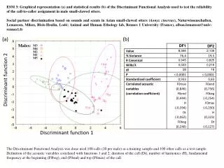
Interpreting discriminant functions • Discriminant function plots – interpret how the functions separate the groups • A visual approach to interpreting the dicriminant functions is to plot each group centroid in a two dimensional plot with one function against another function. • If there are only two functions and they are both statistically and practically interesting, then you put Function 1 on the X axis and Function 2 on the Y axis and plot the group centroids.
2 function plot • Notice how the first function we see all 3 groups distinct • Though much less so, they may be distinguishable on function 2 also Note that for a one function situation we could inspect the histograms for each group along function values
Territorial maps • Provide a picture (absolutely hideous in SPSS) of the relationship between predicted group and two discriminant functions • Asterisks are group centroids • This is just another way in which to see the previous graphic but with how cases would be classified given a particular score on the two functions
Loadings • Loadings (structure coefficients) are the correlations between each predictor and a function. • The squared loading tells you how much variance of a variable is accounted for by the function • Function 1: perhaps representative of ‘country affluence’ (positive correlations on all) • Function 2: Seems mostly related to GDP A is the loading matrix, Rw is the within groups correlation matrix, D is the standardized discriminant function coefficients.
Classification • As mentioned previously, the primary goal in DFA may be geared more towards classification • Classification is a separate procedure in which the discriminating variables (or functions) are used to predict group membership • Up to this point DFA was indistinguishable from MANOVA • In such a situations, we are not so interested in how the variables perform individually per se, but how well as a set they classify cases according to the groups • Prediction over explanation
Equations • Classification score for group j is found by multiplying the raw score on each predictor (x) by its associated classification function coefficient (cj), summing over all predictors and adding a constant, cj0 • Note that these are not the same as our discriminant function coefficients • See mechanics notes
As you can see each group will have a unique set of coefficients and each case will have a score for each group • Whichever one of the groups is associated with the highest classification score is the one the case is classified as belonging to
Alternative Methods • 1. Calculate a Mahalnobis’ distance for each case from a groups’ centroid, and classify it in the group it’s closest to • Would result in a similar outcome as the regular method, though might be useful also in detecting an outlier that is not close to any centroid • 2. One could also use discriminant scores rather than our original variables (replace the xs with fs) • Will generally yield identical results but may not under cases of heterogeneity of variance-covariance matrices or when one of the functions is ignored due non-statistical/practical significance • In this case classification will probably be more accurate as idiosyncratic variation is removed
Probability of group membership • We can also obtain the probability that a case would belong to each group • Sum to 1 across groups • It is actually based on Mahalanobis’ distance (which is distributed as a chi-square with p df) so we can use its distributional properties to assess the probability of that particular case’s value/distance
Probability of group membership • Of course it would also have some probability, however unlikely, of every group. So we assess it’s likelihood for a particular group in terms of its probability for belonging to all groups • For example, in a 3 group situation, if a case was equidistant from all group centroids and its value had an associated probability of .25 for each: • .25/(.25+.25+.25) = .333 probability of belonging to any group (as we’d expect) • If it was closer to one such that • .5/(.5+.25+.25) = .5 for that group and • .25/(.5+.25+.25) = .25 for the others
Prior probability • What we’ve just discussed involves posterior probabilities regarding group membership • However, we’ve been treating the situation thus far as though the likelihood of the groups is equal in the population • What if this is obviously not the case? • E.g. diagnosis of normal vs depressed • We also might have a case where the cost of misclassification is high • AIDS, tumor etc. • This involves the notion of prior probability
Evaluating Classification • How good is the classification? • Classification procedures work well when groups are classified at a percentage higher than that expected by chance • This chance classification depends on the nature of the membership in groups
Evaluating Classification • If the groups are not equal than there are a couple of steps • Calculate the expected probability for each group relative to the whole sample. • For example if there are 60 subjects; 10 in group 1, 20 in group 2 and 30 in group three, then the percentages are .17, .33 and .50. • Prior probabilities • The computer program* will then attempt to assign 10, 20 and 30 subjects to the groups. • In group one you would expect .17 by chance or about 2, • in group two you would expect .33 or about 6 or 7 • and in group 3 you would expect .50 or 15 would be classified correctly by chance alone. • If you add these up 1.7 + 6.6 + 15 you get 23.3 (almost 40%) cases total would be classified correctly by chance alone. • So you hope that you classification works better than that.
Classification Output • Without assigning priors, we’d expect classification success of 33% for each group by simply guessing • And actually by world population they aren’t that far off with roughly a billion members each • Classification coefficients for each group • The results: • Not too shabby 70.7% (58 cases) correctly classified
Output base on priors • Just an example for prior probabilities. • Overall classification is actually worse • Another way of assessing your results is, knowing there were more Catholics (41/84 i.e. not just randomly guessing), my overall classification would be 49% if I just classified everything as Catholic • Is 68% overall rate a significant improvement (practically speaking) compared to that?
Evaluating Classification • One can actually perform a test of sorts on the overall classification • nc = number correctly classified • pi = prior probability of membership • Ni = number of cases for that group • N. = total n
In the informed situation • This ranges from 0 – 1 and can be interpreted as the percentage fewer errors compared to random classification
Evaluating Classification • Cross-Validation • With larger datasets one can also test the classification performance using cross validation techniques we’ve discussed in the past • Estimate the classification coefficients for one part of the data and then apply the coefficients to the other to see if they perform similarly • This allows you to see how well the classification generalizes to new data • In fact, for PDA, methodologists suggest that this is the way one should be doing it period i.e. that the classification coefficients used are not derived from the data to which they are applied
Types of Discriminant Function Analysis • As DFA is analogous to multiple regression, we have the same options for variable entry • Simultaneous • All predictors enter the equation at the same time and each predictor is credited for its unique variance • Sequential (hierarchical) • Predictors are given priority in terms of its theoretical importance, • User defined approach. • Can be used to assess a set of predictors in the presence of covariates that are given highest priority. • Stepwise (statistical) – this is an exploratory approach to discriminant function analysis. • Predictors are entered (or removed) according to statistical criterion. • This often relies on too much of the chance variation that does not generalize to other samples unless some validation technique is used.
Design complexity • Factorial DFA designs • Really best to just analyze through MANOVA • Can you think of a reason to classify an interaction? • However this is done in two steps • Evaluate the factorial MANOVA to see what effects are significant • Evaluate each significant effect through discrim • If there is a significant interaction then the DFA is run by combining the groups to make a one way design • (e.g. if you have gender and IQ both with two levels you would make four groups high males, high females, low males, low females) • If the interaction is not significant then run the DFA on each main effect separately for loadings etc. • Note that it will not produce the same results as the MANOVA would
The causal approach: a summary of DFA • Recall our discussion of Manova
The causal approach • The null hypothesis regarding a 3 group (2 dummy variable) situation. No causal link between the grouping variable and the set of continuous variables.
The causal approach • The original continuous variables are linearly combined in DFA to form y • This can also be seen as the Ys being manifestations of the construct represented by y, which the groups differ on
The causal approach • It may be the case that the groups differ significantly upon more than one dimension (factor) represented by the Ys • Another combination (y*), in this case one uncorrelated with y is necessary to explain the data