Download
1 / 60
600 likes | 701 Views
Random Processes and LSI Systems. What happedns when a random signal is processed by an LSI system? This is illustrated below, where x(n) and y(n) are random signals, and h(n) is a deterministic (i.e., nonrandom) LSI system. x(n). h(n). y(n).

E N D
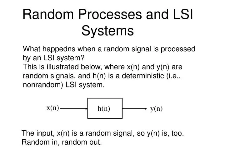
Random Processes and LSI Systems What happedns when a random signal is processed by an LSI system? This is illustrated below, where x(n) and y(n) are random signals, and h(n) is a deterministic (i.e., nonrandom) LSI system. x(n) h(n) y(n) The input, x(n) is a random signal, so y(n) is, too. Random in, random out.
Random Processes and LSI Systems x(n) h(n) y(n) The LSI system, h(n) does exactly the same thing as it would if h(n) were deterministic, so: or, in the frequency domain,
Random Processes and LSI Systems We can take the square of the magnitude, Recall (from the previous lecture) that Sxx(w), the spectral density of x(n), is related to by
Random Processes and LSI Systems so obviously and this can be rewritten as:
Random Processes and LSI Systems so obviously and this can be rewritten as: Since the LSI system is deterministic, we can take it outside the expected value:
Random Processes and LSI Systems What’s left inside the expected value is Sxx(w), so isn’t that nice?
Random Processes and LSI Systems It can be shown that, if x(n) is a zero-mean sequence (which it is) and h(n) is an LSI system (which it is), then y(n) is also zero mean. This means we can find the variance of y (the average output power by: This means we can reduce the average power of a random signal (i.e., reduce the noise power) by attenuating parts of its spectral density function.
Random Processes and LSI Systems The above equation shows that we can attenuate parts of the output noise spectral density by making the system frequency response such that the system rejects those parts. The power of a wideband noise source can be reduced by lowpass (or bandpass) filtering the noise.
Random Processes and LSI Systems Suppose x(n) is a white noise sequence as shown. It’s average power is: Sxx(w) -p p
Random Processes and LSI Systems Now, suppose h(n) is an ideal lowpass filter, wc = p/4 H(w) -p/4 -p p -p/4
Random Processes and LSI Systems So now the output spectral density is this: Syy(w) Sxx(0) -p/4 -p p -p/4 And the average power of the output sequence is:
Random Processes and LSI Systems And the average power of the output sequence is: So reducing the bandwidth by 75% also reduced the noise power by 75%.
Random Processes and LSI Systems Suppose the input to our LSI system h(n) is the sum of two random sequences, z(n) and g(n): z(n) x(n) S h(n) y(n) g(n) If we know Szz(n) and Sgg(n), can we find Syy(n)? Yes!
Random Processes and LSI Systems We already know that So we need to find Sxx(n) in terms of Szz(n) and Sgg(n). recall that: and
Random Processes and LSI Systems Two random processes are independent if the outcome of one does not influence the other. For example, rolling two dice. Two random processes are dependent if the outcome of one can influence the other. Example: drawing a 5-card poker hand.
Random Processes and LSI Systems If the two processes that produce z(n) and g(n) are independent, we can simplify the last expression: and if they’re zero-mean processes, this further reduces to:
Random Processes and LSI Systems and this means that the spectral density of x(n) is So, for two sequences z(n) and g(n), which are generated by independent, zero-mean random processes, summed together to form the input sequence x(n) to an LSI system h(n), the output noise spectral density is
Random Processes and LSI Systems Finally, the average power of the output sequence y(n) is:
White Noise A zero-mean white noise sequence x(n) has the following proprerties: E[x(n)] = 0 x(k) and x(k+n) are independent if n is nonzero. White noise is independent with respect to any other sequence.
White Noise If two random variables x and y are independent, So, for white noise, But E[x(n)] = 0, so
White Noise We’ve previously seen that So we’ve just shown that for white noise, The power spectral density is the DTFT of the autocorrelation function, so for zero-mean white noise, which is constant across the entire spectrum (white).
White Noise We can generate a zero-mean white noise sequence x(n) by randomly choosing, for each n, a real number between –D/2 and D/2. Each number must be independent of the choice of all others. This is a uniformly distributed, zero mean, white noise signal.
Quantization Noise and Oversampling Here’s a VERY practical example of exactly this type of signal: quantization noise. Suppose we have an N-bit A/D converter with an input we designate xa(t). xa(t) can range from a minimum of -V volts to a maximum of +V volts. The A/D converter samples xa(t) every T seconds, and produces an N-bit binary number which approximates the quantized value of the sample xa(nT)
Quantization Noise and Oversampling An N-bit binary number is used to represent the sampled input, xa(nT). This binary number has a finite number of possible values: 2N. Each of these values represents a range of possible input voltages, and there is one such range for each possible N-bit number. Thus, the total input range, is divided into 2N smaller ranges.
Quantization Noise and Oversampling Each of these smaller ranges can be expressed as where M is the actual N-bit number representing a particular sample. The following figure illustrates these relationships for a 4-bit A/D converter (N = 4).
Quantization Noise and Oversampling M xa M=1 M=0 4-bit A/D converter
Quantization Noise and Oversampling If the output of the A/D converter is M, xa(nT) is somwhere in the range So, if the output of the A/D converter is M, this says that the input is
Quantization Noise and Oversampling If the output of the A/D converter is M, xa(nT) is somwhere in the range So, if the output of the A/D converter is M, this says that the input is
Quantization Noise and Oversampling If we let the A/D converter output be the center of the range, we can rewrite the previous relationship as
Quantization Noise and Oversampling or where x(n) is the actual input signal to the A/D converter, and the A/D output is We can express the quantization error as an error (or noise) sequence, e(n), yielding this:
Quantization Noise and Oversampling Written this way, The A/D converter’s output can be thought of as the sum of two sequences: a signal sequence equal to the input signal sampled by an ideal, infinite-precision A/D converter, and the quantization noise sequence, e(n). Note that the quantization noise can have any value between –D/2 and D/2, and its probability density function is uniform.
Quantization Noise and Oversampling Consider the signal sequence, x(n). It’s average power is The quantization noise sequence has this average power: so the A/D converter’s signal to noise ratio (SNR) is:
Quantization Noise and Oversampling We can write the SNR in terms of decibels: Naturally, we want the SNR to be as large as possible. This means we make the signal power as large as possible, by using the entire input range of the A/D converter. We also minimize the noise power. One way to do this is to increase the number of bits, which may or may not be practical. We would like to have another way.
Quantization Noise and Oversampling To see if there is another way, let’s investigate e(n). We know that e(n) is a random variable with values in the range and it’s uniformly distributed in that range. Positive and negative values are equally likely, so it’s a zero-mean process.
Quantization Noise and Oversampling It’s average power is:
Quantization Noise and Oversampling With this knowledge, we can write the SNR as Or, in dB:
Quantization Noise and Oversampling If N > 8, we can use this approximation: substituting this in the previous expression for SNR gives us:
Quantization Noise and Oversampling Which shows that each additional bit of precision improves the SNR by about 6 dB. This makes sense, since it cuts D in half. It’s not too much of a stretch to assume that quantization errors occurring at different times are independent. If this is assumed, then the quantization noise sequence, e(n), satisfies the conditions to be modeled as uniformly distributed white noise.
Quantization Noise and Oversampling We’ve already seen that the power spectral density of a white noise sequence x(n) is so the power spectral density of e(n) is as shown below: See(w) se2 -p p
Quantization Noise and Oversampling So the average power of the quantization noise sequence e(n) is spread over the discrete time frequency range from –p to p. Remember that p radians per sample in the discrete time domain maps to fs/2 in the continuous time domain, so the quantizing noise power is spread over the range – fs/2to fs/2. See(2pfT) se2 - fs/2 - fs/2
Quantization Noise and Oversampling If, for example, we quadruple the sampling frequency, but leave N alone, we take the quantizing noise power and spread it over a band four times as wide. Suppose we have a bandlimited signal (bandwidth = B) with power spectral density shown in the next slide:
Quantization Noise and Oversampling Sxx(f) A f -B B If we sample it at the minimum sample rate, fs = 2B, the spectral densities of the signal sequence and the quantization noise sequence are as shown next:
Quantization Noise and Oversampling Sxx(f) 2BA se2 f -p p If we double the sample rate (fs = 4B), the signal and noise spectral densities are as shown:
Quantization Noise and Oversampling Sxx(f) 4BA se2 f -p -p/2 p/2 p If we double the sample rate again (fs = 8B), the signal and noise spectral densities are as shown:
Quantization Noise and Oversampling Sxx(f) 8BA se2 f -p -p/4 p/4 p Note that the true signal power and the true noise power are the same in all three, the apparent difference merely serves to show that the noise power is spread over a wider band.
Quantization Noise and Oversampling This can be generalized for fs = 2MB, as shown below: Sxx(f) 2MBA se2 f -p -p/M p/M p Notice that if M > 1 (i.e., if the signal is oversampled) some of the noise power is outside the signal bandwidth.
Quantization Noise and Oversampling We can eliminate the portion of the noise power which is outside the signal bandwidth by using a digital lowpass filter to attenuate it. Since this filter will not attenuate anything in the signal band, the signal (and the information it conveys) is unaffected. Unfortunately, the in-band noise is also not affected, but getting rid of the out-of-band noise is a good thing.
Quantization Noise and Oversampling If M, the oversampling factor, is 1, we are sampling at the minimum rate, and the SNR is given by If we let M = 2 (oversampling by a factor of 2), and use an ideal lowpass filter to eliminate out-of-band noise, the result is as shown next:
Quantization Noise and Oversampling Sxx(f) 4BA se2 f -p -p/2 p/2 p This eliminates half the noise power, doubling the signal to noise ratio. If we let M = 4 (oversampling by 4), the SNR is doubled again: