Download
1 / 47
480 likes | 801 Views
Workshop XX Transonic Flow over a RAE 2822 Airfoil. Introductory FLUENT Training. Goals. The purpose of this tutorial is to introduce the user to good techniques for modelling flow in high speed external aerodynamic applications

E N D
Workshop XXTransonic Flow over a RAE 2822 Airfoil Introductory FLUENT Training
Goals The purpose of this tutorial is to introduce the user to good techniques for modelling flow in high speed external aerodynamic applications Transonic flow will be modelled over a RAE 2822 airfoil for which experimental data has been published, so that a comparison can be made The flow to be considered is compressible and turbulent The used solver is the density based implicit solver The tutorial is carried out using FLUENT and CFD Post from within Workbench, but it could also be completed in standalone mode
Task Description Simulation Goals Drag and Lift Coefficient Flow Field Ma number Pressure CL? CD? a Ma = 0.75 pstatic = 11111 Pa Tstatic = 216.65 K a = 3,19°
Start FLUENT Stand-alone Start a Stand-alone FLUENT session: Start/All Programs/ANSYS12.0/Fluid Dynamics/Fluent Or use the Short Cut (Windows)
Start FLUENT Stand-alone Start a Stand-alone FLUENT session: Launch a 3D, double precision, serial session
Import the mesh • Import the mesh file • File/Read/Mesh/ • Select the mesh file rae2822_coarse.msh
Mesh The mesh will read in and display Rotate the mesh so you can see the mesh like shown below
Mesh (2) • Select General > Scale and observe the current domain extents • Check that the domain extents are as expected. • Select General > Check and check there are no errors • Finally use ‘Report Quality’ to print out cell quality statistics
Mesh (3) Zoom in and examine the mesh The maximum aspect ratio in this mesh is quite high (around 7000) This is acceptable because these cells are close to the airfoil wall surfaces This is needed for the turbulence model being used, since it ensures the first grid point is in the viscous sublayer
Solver • Select the steady-state implicit density-based solver • From ‘General’ in the tree check Type: Density-Based • Check time is steady • Turn on the energy equation • This is needed because the flow is compressible and we will be using the ideal gas equation • Select the turbulence model to be used • From ‘Models’ in the tree, select ‘Viscous’ and Edit • Choose the two-equation SST-k-omega model
Materials • The properties to be used for the material ‘air’ need to be set • For Density, select ‘Ideal Gas’ • For Viscosity, select “Sutherland”, and accept the default settings for the 3 Coefficient method • The Sutherland law for viscosity is well suited for high-speed compressible flow. For simplicity, we will leave Cp and Thermal Conductivity as constants. Ideally, in high speed compressible flow modeling, these should be temperature dependent as well • Select Change/Create • Assign the material ‘air’ to the grid cells • Select ‘Cell Zone Conditions’ • Highlight ‘fluid’ then ‘Edit’ • Observe ‘air’ is already selected
Operating Conditions • Set the Operating Pressure to Zero • Absolute pressure is the gauge pressure plus the operating pressure • Setting zero operating pressure means that all pressures set in FLUENT will be absolute • This is the most common practice for compressible flows • Select ‘Cell Zone Conditions > Operating Conditions • Set the Operating Pressure to Zero, then ‘OK’
Boundary Conditions - inlet • Select ‘Boundary Conditions’ • Set inlet to type pressure-far-field • Pressure far-field conditions are used in ANSYS FLUENT to model a free-stream condition at infinity, with free-stream Mach number and static conditions being specified • It is a non-reflecting Boundary Condition • Use • The pressure-far-field boundary type is applicable only when the density is calculated using the ideal-gas law • It is important to place the far-field boundary far enough from the object of interest. For example, in lifting airfoil calculations, it is not uncommon for the far-field boundary to be a circle with a radius of 20-50 chord lengths
Boundary Conditions - inlet • On the ‘Momentum’ tab • set the gauge static pressure to 11111 Pa • This value is used to calculate the total pressure based on the MA number • Set the Mach Number to 0.75 • The angle of attack (α) in this numerical case is 3.19 deg. • The x-component of the flow is cosα (0.99845) • The z-component of the flow is sinα (0.05565) • It is common practice to adjust the numerical α from the experimental α in order to match the lift obtained in the wind tunnel, and then to determine the drag associated with this lift. This adjustment of α is carried out to counter the effects of the wind tunnel enclosure. • Select ‘Intensity and Viscosity Ratio’ • Set Turbulent Intensity to 1% • Set Turbulent Viscosity Ratio to 1
Boundary Conditions - inlet • Select the Thermal tab • Set the Static Temperature to be 216.65 K • The total Temperature is calculated based on the Ma number
Boundary Conditions – airfoil & symmetry For the boundary airfoil select type wall Leave the default settings which correspond to a no-slip condition for momentum and adiabatic (Heat flux = 0) for thermal For the boundary symmetry select the type symmetry No further settings possible
Reference Values • Set the reference values as shown: • These are not used in the actual solution, but are used for reporting coefficients, such as CL and CD. Infinite BC
Solution Methods • Select Solution Methods in the LHS tree • Keep the default settings for the implicit formulation and Roe-FDS flux type • This will enable the Density-based Coupled Implicit Solver • The Density-based Coupled implicit formulation is more stable and can be driven much harder to reach a converged solution in less time • The Density-based Coupled explicit formulation is only normally used for cases where the characteristic time scale is of the same order as the acoustic time scale, for example the propagation of high Mach number shock waves
Solution Methods • Change the gradient method to Green-Gauss Node Based • This is slightly more computationally expensive than the other methods but is more accurate • Select Second Order Upwind for flow and turbulence discretization • To accurately predict drag, select the ‘Second Order Upwind’ schemes.
Solution Controls • The Courant number (CFL) determines the internal time step and affects the solution speed and stability • The default CFL for the density-based implicit formulation is 5.0. It is often possible to increase the CFL to 10, 20, 100, or even higher, depending on the complexity of your problem. You may find that a lower CFL is required during startup (when changes in the solution are highly nonlinear), but it can be increased as the solution progresses As we will be using automatic ‘solution steering’, the choice of CFL at this stage is not important for this case Keep the default under-relaxation factors (URFs) for the uncoupled parameters
Solution Monitors - Residuals • Set up residual monitors so the convergence can be monitored • Monitors > Residuals > Edit • Make sure ‘plot’ is on • Turn off convergence checks by setting the criterion to ‘none’ • This means that the calculation will not stop based on the residual plots convergence, but you can still see their progress.
Solution Monitors – Drag & Lift • Set up a monitor for the drag coefficient on the airfoil. • Select both wall zones and toggle on ‘Print’, ‘Plot’ and ‘Write’. • Remember that α is 3.19° so we need to use the force vector as shown • Lift and drag are defined relative to the wind, not the airfoil • Press OK, then follow the same process to setup a monitor for Lift • The settings are identical except for the File Name (cl-history instead of cd-history) and the Force Vectors: -0.0556 as x component and 0.99845 as z component
Solution Initialization Initialize the flow field based on the far-field boundary Select Solution Initialization from the model tree Compute from > inlet Press ‘Initialize’
Solution Steering Enable the Solution Steering option Select Run Calculation, and toggle on Solution Steering Change the flow type to transonic and keep default options Click on Use FMG Initialization Full-Multi-Grid Initialization will compute a quick, simplified solution based on a number of coarse sub-grids. This will then be used as a starting point for the main calculation. FMG initialization can help to get a stable starting point • Solution Steering enables the robust first order discretization in the early-stages of the computation, then blends to the more accurate second order schemes as the solution stabilizes
Case Check • Check the case file and make sure there are no reported issues • Use Run Calculation > Check Case • Any potential problems with the case setup will be raised in the case check panel if there are no problems this panel will not appear. In this case there is a recommendation to check the reference values for the force monitors. Since we have already set these we can ignore this warning.
Save the Case File • Save the case file • File > Write Case • You can write case and data files with extension .gz – the files will be compressed automatically
Run Calculation – FMG Initialization (1) Although the calculation is ready to compute, It is good practice (but not strictly necessary) to run the FMG initialization and then check the coarse FMG solution before starting the main calculation iterations Set the number of requested iterations to zero, and press ‘Calculate’ or input /solve/init/fmg at TUI Do it twice!
Run Calculation – FMG Initialization (2) Check the pressure and velocity contours Go to ‘Graphics and Animations’ in the LHS tree, choose ‘Contours’ and ‘Set Up’ Choose Contours of Pressure > Static Pressure, ‘Filled’ Option and select the Surface ‘symmetry’ Display (If you need to autoscale the display, press <control> A) Repeat for Contours of Velocity> Mach Number Ma P
Run Calculation (1) There are no spurious results from the FMG Initialization, so proceed to the main calculation Return to ‘Run Calculation’ in the LHS tree Disable ‘Use FMG Initialization’ Change the number of windows to three for the residual, drag and lift monitors that we set up earlier (see disposition on next slide) Request 900 iterations ‘Calculate’
Run Calculation (2) • After 900 iterations the calculation has fully converged • Note that the CFL has been updated during the calculation in a number of stages, ramping up from 5 to 200 (as requested by default). This can be seen in the CFL window and the effect on the residuals is also evident • By the end of the calculation the residuals have converged well and are no longer changing. The drag and lift monitors are also stable • It can be observed that the Residuals of Y-velocity is quite high. This is not a problem because this simulation is a 2d analysis on the XZ plane, on Y-direction there is only one layer of cells and the flow field in that direction is not of interest !
Save the Case&Data Files • Save the Case&Data files • File > Write Case&Data.. • You can write case and data files with extension .gz – the files will be compressed automatically
Post Processing – Data Export • Additional post-processing will now be performed in CFD Post • Export the data in CFD-Post compatible Format • You can specify which values you will have for Post-processing • Velocity Magnitude and Components • Mach Number • Pressure • Click on ‘Open CFD-Post’ to automatically start a CFD-Post session • Close FLUENT (File > Exit)
CFD-Post Define the Post-processing view • Right-click on a blank area of the screen and select Predefined Camera>View Towards –Y • Use the box zoom so the viewer displays the region around the airfoil
CDF-Post When looking at the flow around an airfoil, plots of several variables can be of interest such as velocity, pressure, and Mach number • In the tree turn on the visibility of symmetry by clicking in the tick box the double click on it to bring up the details section • Under the Colour tab change the mode to Variable and select Velocity using the Global Range, then click Apply. Notice that the maximum velocity is around 354 m/s
CFD-Post To plot Mach number a contour plot will be used so the supersonic region can clearly be identified • Select Insert>Contour or click on the contour icon • Accept the default name then set Locationto symmetry and the Variable to Mach Number • Change the Range to User Specified and enter 0 to 1.33 as the range • Set # of Contours to 21, the click Apply
CFD-Post • To have some further variables available (Pressure Coefficient, Lift Coefficient, …) we need some Expressions • Read these with File > Load State expressions.cst • Now you can see the Definitions in the Expression Tab
CFD-Post To plot the pressure coefficient distribution around the airfoil a polyline is needed to represent the airfoil profile and a variable needs to be created to give CP • Create a Polyline using Insert>Location>Polyline • Change the Method to Boundary Intersection • Set Boundary List to Airfoil, Intersect With to Sym 1 then click Apply • A line will be created around one end of the airfoil • For full 3D cases other locations could have been extracted if a XY plane was first created
CFD-Post 4. Move to the Variables tab and enter a variable MyCP - Set the Method to Expression and select CP
CFD-Post A chart showing the pressure distribution around the airfoil will now be created • Insert a chart using Insert>Chart or selecting . • In the General tab leave the type as XY • Move to the Data Series tab and enter a new series - Set the location to Polyline 1 • Move to the X Axis tab and change the variable to X • Move to the Y Axis tab and change the variable to MyCp - Invert Axis selected • Click Apply and the chart is generated These values can be compared with experimental results • Return to the Data Series tab and change the name to FLUENT • Insert a new series and give it the name Experiment • Change the Data Source to File and select ExperimentalData.csv • Click Apply and both lines are drawn
Summary In this tutorial we have used FLUENT to compute the transonic, compressible flow over a RAE 2822 airfoil We have used the density based solver with solution steering We have seen how FLUENT can be linked to CFD Post, and we have explored some of the features within CFD Post We have compared the results to published experimental data Next step could be to use medium and fine mesh – Grid dependency of solution?
References AGARD 138; Test Case 13A Airfoil RAE 2822 – Pressure distributions and boundary layer and wake measurements; Cook, McDonald, Firmin
Post Processing [FLUENT] • Select ‘Graphics and Animations’ in the LHS menu • Examine the contours of static pressure. • Turn off ‘Filled’ to just display the contour lines • Adjust the Levels to increase the number of contour lines The contour will display in the active window (click a window to activate). Alternatively, use the drop down menu to return the display to a single window as shown here
Post Processing [FLUENT] Plot contours of Velocity > Mach Number and notice that the flow is now locally supersonic
Post Processing [FLUENT] Select ‘Plots’ in the LHS menu Plot Pressure Coefficient along the airfoil surface
Post Processing [FLUENT] Once loaded, plot the CFD and experimental Cp (experiment.xy) plots together A good agreement can be seen
Post Processing [FLUENT] • Compare the predicted CL and CD against the experimental values. • From Reference • CL = 0.733 and CD = 0.018 • From the console window, we have predicted • CL = 0.746 and CD = 0.0287 • ReasonforDifference? • Wall interference > effective angel ofattack 2.82°