Download
1 / 27
290 likes | 445 Views
Optimal Design of Qualitative Risk Matrices to Classify Quantitative Risks. Bill Huber Quantitative Decisions Rosemont, PA Tony Cox Cox Associates Denver, CO. Outline. Setting the Scene Examples : risk matrices are widely used.

E N D
Optimal Design of Qualitative Risk Matrices to Classify Quantitative Risks Bill Huber Quantitative DecisionsRosemont, PA Tony Cox Cox AssociatesDenver, CO
Outline • Setting the Scene • Examples: risk matrices are widely used. • Definitions and terminology: our model applies to most risk matrices. • Pros and cons of risk matrices: they have their uses, but problems lurk. • The Risk Matrix Design problem: if you must create a risk matrix, how well can you do and is it worth the effort to do a good job? • Optimal Risk Matrix Design Theory and Results (Binary Case) • Result 1: Make your matrices as square as possible. • Result 2: Create the best matrix with the Zig-Zag construction. • Further Research • Beyond binary: What about risk matrices with more than two decisions? • What you can do. Quantitative Decisions/Cox Associates
Risk Matrices Swedish Rescue Service Canadian Navy U.S. FHA Supply Chain Digest Australian Government Quantitative Decisions/Cox Associates
Definitions • A risk matrix assigns a unique decision to any prospect: • Accounts that could go bad; • Facilities that might be attacked; • Research, development, or exploration projects that might not come to fruition; etc. • It presents a two-dimensional table of decisions. • Rows correspond to classes (or “bins”) of a prospect attribute u (typically consequence, severity, impact, or disutility) and columns to bins of another attribute p (typically probability). • u and p might be computed from other prospect attributes. • Decisions could be • Act now, take risk mitigation countermeasures, perform a follow-on study: typically colored red. • Do nothing, act later, assume no risk: typically colored green. Quantitative Decisions/Cox Associates
Uncovering the Detail (From a consultant’s white paper) Harvard Business Review Pêches et Océans Canada Quantitative Decisions/Cox Associates
Risk Matrices Are DiscreteApproximations • Their creators clearly conceive of risk matrices as discrete representations of functional relationships. • Thus, • Columns bin the values of p at breakpoints x0 (the smallest possible value of p), x1, x2, …, xn (the largest possible value). • Rows bin the values of u at breakpoints ym < ym-1 < ym-2 < … < y0. • Risk is determined by a function v(p,u): the valuation function. (Often p and u can be expressed so that v(p,u) = pu: “risk is probability times consequence.” However, p does not need to be probability, nor does u have to be consequence, and our theory handles a large class of valuation functions besides pu.) • Decisions are intervals of risk (z0,z1], (z1,z2], …, (zL-1,zL]. Quantitative Decisions/Cox Associates
Notation column j u axis prospect (p,u) Bin (yi, yi-1] for u:yi< u yi-1. row i The decision for prospect (p,u) is shown here as aij. We talk about it generically as a color ranging from green through red. p axis Bin (xj-1, xj] for p:xj-1 < p xj. Quantitative Decisions/Cox Associates
Why Use Risk Matrices? • The risk attributes p and u or the valuation function v(p,u) might not be accurately known or precisely measurable. • Computing v(p,u) and comparing it to the breakpoints z1, z2, …, zL-1 may be burdensome, time consuming error prone, or could reveal sensitive information. • When p or u change frequently, a risk matrix expedites the response. • A risk matrix can present, simplify, and document the information used to make a decision. Quantitative Decisions/Cox Associates
Problems with Risk Matrices • Binning (classifying into categories) the variables p and u almost always loses some information that may be needed for correct decision making. • This causes the risks of some pairs of prospects to be ranked incorrectly. • It is possible for decisions made with them to be worse than random! (LA Cox Jr, What’s Wrong with Risk Matrices, Risk Analysis 28(2), 2008). • An error will occur when a prospect with attributes (p,u) falls into a cell whose color is not the correct one for the “true” risk v(p,u). We call these the “bad” prospects for the risk matrix. • “Gray” cells by definition contain both good and bad prospects. • How bad can the errors get in actual use? Quantitative Decisions/Cox Associates
The Risk Matrix Design Problem • Given a valuation function v(p,u) and constraints (upper bounds) on the numbers of rows and columns you want to use, determine breakpoints x1, x2, …, xn-1; y1, y2, …, ym-1; and z1, z2, …, zL-1 that minimize the “overall” error made by users of the risk matrix. • In most cases, the set of decisions is predetermined, thereby fixing the breakpoints z1, z2, …, zL-1. • “Overall” error can be measured in several ways, including maximum possible error, expected error under a probability distribution of prospects, or expected error rate. • How well can an optimal matrix perform compared to an “intuitive” or “generic” solution? Quantitative Decisions/Cox Associates
Theory and Results The Case of Binary Risk Matrices
Preliminaries • Re-expressp and u so they both lie in the interval [0, 1]. • There is no loss of generality: ultimately both variables will be binned anyway. • Assume v(p,u) is strictly increasing in both arguments in the interior of its domain (i.e., (0,1) (0,1)). • This is natural: anything else probably doesn’t qualify as a valuation function. • A binary (two-decision) problem divides prospects into “green” ones where v(p,u) k and “red” ones where v(p,u) > k. (k is known as “acceptable risk.”) • The threshold k is fixed. It determines the decision curve {(p,u) : v(p,u) = k}. • Adopt a cost functionC(p,u,d). The cost is that of making decision d for prospect (p,u). Often, C will indicate error or the size of the error. • When the decision is the correct one, the cost is zero. • E.g., relative risk is C(p,u,d) = |v(p,u) – k|. Indicator risk is C(p,u,d) = 1. • Optionally specify a probability (or frequency) distribution for the prospects. • E.g., the uniform distribution d = dpdu. Quantitative Decisions/Cox Associates
Two Kinds of Problems • The minimax problem is to optimize the worst cost that can be incurred in using the risk matrix. • The expected cost (or expected loss) problem is to optimize the average cost incurred in using the risk matrix. • This requires one to specify the frequencies (or probabilities) with which the prospects will occur. • For either problem, • Use indicator riskC(p,u,d) = 1 to measure error rates. • We use relative riskC(p,u,d) = |v(p,u) – k| to account for the degree of error as well as its occurrence. • Generally, the cost should increase or at least stay the same as the difference between the risk matrix’s prescription and the true decision increases. We solve the problem in this most general setting. Quantitative Decisions/Cox Associates
Binary Risk Matrices • Binary risk matrices have two colors only: red and green. • Understanding them is a key step towards a general theory of optimal risk matrix design. Műnchener Rűck Munich Re Group Quantitative Decisions/Cox Associates
Choosing the Right Decisions • After binning the variables, you can go cell by cell through the matrix to pick the decision that minimizes the cell’s cost. • When all prospects in the cell have the same color, give the cell that color (obviously). • Otherwise • In the minimax problem, consider the worst prospect for each possible cell color. Choose the color that minimizes this worst case. • In the expected cost problem, choose the color that minimizes the expected cost over the cell. • Thus, the problems of choosing breakpoints and coloring the cells are decoupled. However we color this gray cell, the worst costs will be incurred at the two corner cells marked. In solving the expected cost problem, we have to integrate the cost over the upper half of the cell (if it’s colored green) or over the lower half (if it’s colored red). Quantitative Decisions/Cox Associates
We prove there is a unique point in the sweep where the sum of the two costs is smallest. The cost of this cell goes up … while the cost of this cell goes down. Sweeping through a Strip • Focus on one column as you vary one y-breakpoint. The colored dots mark curvilinear triangles containing bad prospects. E.g., the cell for the green dot (at the left) will necessarily be colored red, but this prospect—lying below the decision curve—is green. Quantitative Decisions/Cox Associates
The Key Idea • At any critical point, the infinitesimal increase in cost contributed by the green (left) line segment balances the infinitesimal decrease in cost contributed by the red (right) line segment. Quantitative Decisions/Cox Associates
Result 1: Use Square Matrices • Make the matrix as square as possible (that is, m and n should be equal or differ by one). • If not, there will be neighboring rows (or columns) that can be combined without any increase in overall cost. No matter how we vary y2 between y1 and y3, the row of cells between y1 and y2 must always be colored the same as the row of cells between y2 and y3. Thus, y2 is unnecessary. This situation always happens when there are more rows than columns+1. Quantitative Decisions/Cox Associates
Result 2: The Zig-Zag Procedure • The “zig-zag” procedure always produces a best set of breakpoints. • This works for any reasonable cost function C and valuation v. • It applies to expected cost and minimax cost. • The procedure: • Start at top (or left). • Move down (or right), cross the decision curve, and move an “equivalent” distance beyond it. • Make a right turn. • Repeat until you move beyond the square. • If your last step lands exactly on the boundary, you have a good design. • This produces a set of simultaneous equations we can solve explicitly. Quantitative Decisions/Cox Associates
How Good Is Best? • The graphic shows how overall costs for relative risk vary with breakpoints in a binary 2 2 risk matrix. • The problem’s symmetry (correctly) suggests the y breakpoint should equal the x breakpoint. • Here, poor choice of breakpoints can increase losses over 100% (minimax) or almost 400% (expected loss, uniform distribution) relative to the best choice. Note the logarithmic scale for loss (overall cost). Quantitative Decisions/Cox Associates
How Good Is Best? (2) • The “naïve” design divides p and u each into n equally spaced bins (which is often done). • These values of k are the worst case for v = pu: for them, the minimax cost is largest. • Nevertheless, the “Ratio” column shows the best design is typically 2.5 to 3 times better than the naïve one. • Similar results hold for the expected-cost problem. Maximum Relative Risk n k Naïve Optimal Ratio 2 0.3750 0.1250 0.1250 1.00 3 0.3704 0.1481 0.0741 2.00 4 0.3691 0.1309 0.0527 2.48 5 0.3686 0.1114 0.0410 2.72 6 0.3684 0.0906 0.0335 2.71 7 0.3682 0.0621 0.0283 2.19 8 0.3682 0.0693 0.0245 2.83 9 0.3681 0.0718 0.0217 3.32 10 0.3680 0.0520 0.0194 2.68 11 0.3680 0.0452 0.0175 2.58 12 0.3680 0.0487 0.0160 3.04 13 0.3680 0.0462 0.0147 3.14 14 0.3680 0.0414 0.0136 3.04 15 0.3680 0.0365 0.0127 2.88 n = #rows, #columns. k = decision threshold.“Naïve” and “Optimal” are maximum relative risk errors caused by using a risk matrix. Quantitative Decisions/Cox Associates
Further Research Beyond Binary Risk Matrices
What Next? • What can we say about more than two decisions? • The strip sweep analysis still works. • The Zig-Zag procedure does not easily extend to more than two decisions because of interactions between strips. • It is unlikely we will find any simple, clear characterization of all optimal risk matrices. • What can we say about arbitrary probability distributions of prospects? • Not much, unless we make strong assumptions. • Nevertheless, our results for the binary case suggest significant improvements over intuitive or naïve designs are possible. • The Zig-Zag procedure applied independently to the L-1 cutoffs for an L-decision matrix might be a good heuristic guide in many cases. Quantitative Decisions/Cox Associates
What You Can Do • Consider using the Zig-Zag procedure to help determine cutoffs for p and u in your risk matrices. • More generally, evaluate the potential effects of a risk matrix in terms of the maximum error or expected error incurred by its users. • If your analysis suggests the error rates are unacceptable, you can • Increase the numbers of rows and columns or • Provide quantitative decision procedures (formulas) or software in place of a risk matrix. Quantitative Decisions/Cox Associates
QD and CA Supporting you and solving your problems with maps, numbers, and analyses. www.quantdec.com Superior business decisions through better data analysis. www.cox-associates.com
Finding the Best Breakpoints • The overall cost of the design, given that we have selected the best color for each cell, is a function of n+m–2 variables subject to the constraints 0<x1<x2 …<xn-1<1>y1>y2>…>ym-1>0. • For the minimax problem the cost is not differentiable (vide the red curve) so we have to be careful about using Calculus. • Nevertheless, we can use the fundamental idea of looking for the best design at critical points where independent small changes in any variable no longer improve the cost. • Changing any variable causes changes in the strips of cells through which it passes. Therefore, we study how the cost changes as a breakpoint sweeps across one strip. Quantitative Decisions/Cox Associates
Example:Minimax relative risk for v = pu For an n by n risk matrix with decision threshold k, valuation function v(p,u) = pu, and relative risk cost c(p,u,d) = |v(p,u) – k| (when d is the wrong decision for (p,u)), maximum loss is minimized uniquely by choosing breakpoints in the zig-zag construction beginning at x1 = k + e where e is the only positive root of (k + e)n = (k – e)n –1. The x-breakpoints lie in geometric progression with common ratio r = (k+e)/(k–e), so that xi = (k + e)r i‑1 = (k + e)i / (k – e)i‑1, i = 1, 2, …, n. The y-breakpoints are the same as the x-breakpoints. The maximum loss is e. For k = 0.25 and m = n = 4, e 0.039. Note that 0.289 = 0.25 + 0.039 and 0.211 = 0.25 – 0.039. Quantitative Decisions/Cox Associates