Traffic Management

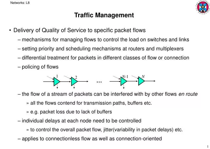
Networks: L8 Traffic Management • Delivery of Quality of Service to specific packet flows • mechanisms for managing flows to control the load on switches and links • setting priority and scheduling mechanisms at routers and multiplexers • differential treatment for packets in different classes of flow or connection • policing of flows • the flow of a stream of packets can be interfered with by other flows en route • all the flows contend for transmission paths, buffers etc. • e.g. packet loss due to lack of buffers • individual delays at each node need to be controlled • to control the overall packet flow, jitter(variability in packet delays) etc. • applies to connectionless flow as well as connection-oriented 1 N-1 N 2 …

Networks: L8 • FIFO and Priority Queues • First-In-First-Out: all arriving packets placed in a queue • transmitted in order of arrival • packets discarded when buffer full: • higher protocol level can deal with any retransmission • delay and loss of packets depends on interarrival times and packet lengths • the more bursty the flow or with packet lengths more variable, the more performance deteriorates • subject to hogging • when one flow sends packets at a high rate and fills all the buffers • depriving other flows of access to the transmission system • not possible to provide differentiated services in basic FIFO scheme • since all packets treated in the same fashion • different services can be provided with a FIFO variation with priority classes: • packets from the higher priority class are buffered as long as there is space • packets from the lower priority class are discarded when number of packets buffered reaches a threshold Packet buffer Arriving packets Packet discard when full

Networks: L8 Packet discard when full High-priority packets Transmission link Low-priority packets When high-priority queue empty Packet discard when full • Head-of-Line priority queuing: • separate queues for each of a number of priority classes: • high priority queue for packets with low delay requirements and vice versa • size of buffers for different priority classes according to loss probability needs • pre-emptively always select next packet from highest priority queue • can lead to starvation of lower priority queues • or allow a flow of packets from lower priority queues at less frequent rates • etc. as in OS process and real-time scheduling • still no discrimination between flows at same priority level • hogging can still occur

Networks: L8 • Sorted packet queuing • queue sorted in order of some priority tag • but still discard when buffers full • defining priority can be very flexible • could be dynamic as conditions and flows change • e.g. tagged with a priority class and arrival time • effective priority increasing with time as the packet delayed • priority could reflect a time due • the time by which the packet should be transmitted • packets with no delay requirement get indefinite or long times-due • time-critical packets get a short time due Sorted packet buffer Arriving packets Tagging unit Transmission link Packet discard when full

Networks: L8 • Fair Queueing • attempts to provide equitable access to transmission bandwidth • each packet flow has its own queue • bandwidth could be divided equally between flows • each flow transmitted in turn in round robin fashion: • in practice flows may get better than an equal share • since some queues will periodically be empty with irregular traffic • flows can be interleaved at either the packet level or a lower level e.g. byte • byte interleaving effectively reduces the flow rate for each flow • packet interleaving introduces delays to some packets i.e. jitter Packet flow 1 round robin service Packet flow 2 Transmission link Packet flow n

Networks: L8 • with packet interleaving, bandwidth not necessarily equally shared • packet lengths of different flows may vary • flows with larger packet sizes will get more of the bandwidth • like interactive versus CPU bound processes in an OS • short interactions do not take all their allocated time-slice • CPU bound processes take their full time-slice • a fairer system takes packet length into account • each time a packet arrives, it is tagged with a transmission finish time for the packet which represents it getting a fair share of the bandwidth • fair share of bandwidth = transmission capacity / number of flows • for a packet arrival with its flow queue currently empty, finish tag is packet length / fair share of bandwidth • into the future from its arrival time • for a packet arrival with its queue not empty, the finish tag of the preceding packet must be added in • or could be calculated when the previous packet has completed transmission

Networks: L8 • each time a packet transmission is complete, the next packet to be transmitted is the one with the closest finish tag • guarantees a flow at least its fair share of bandwidth • but not a guarantee of absolute Quality of Service • that depends on the number of flows grabbing their share • actual transmission completion time for a packet will vary depending on whether any other queues are empty • for byte-by-byte interleaving of packets, the start of transmitting a packet could be delayed depending on its past usage of bandwidth • sorting out which byte belongs to which packet at the other end a problem • only sensible for a constant number of flows • then wastes slots when no packets queued for a certain flow • Weighted Fair Queueing • when flows have different delay requirements • a weight can be applied to each flow to calculate a fair share of bandwidth • if flow i has a weight wi, its proportion of the bandwidth = wi / w

Networks: L8 • Quality of Service (QoS) in the Internet • to support real-time applications such as audio and video, Internet must provide some level of QoS • can be a differentiated service • some classes of traffic treated preferentially relative to other classes • can be charged for accordingly • packets are marked at the edge of the network to indicate the type of treatment they should receive at all the switches in the network • but this does not provide a strict QoS guarantee • to give a guaranteed QoS • e.g. that gives a strict bound of the end-to-end delay for all packets • resource reservations must be made along the path • a connection-oriented service • negotiations take place with each network switch to reserve bandwidth • weighted fair queuing plus traffic regulation are needed to provide this • ATM networks offer this kind of service

Networks: L8 Controlled Throughput Uncontrolled Offered load Congestion Control • congestion occurs when too many packets arrive at the same switch • if the arrival rate can be greater than the onward transmission rate • the pool of buffers in the switch can be used up • can happen irrespective of how big the pool is • a larger pool just postpones the congestion • when buffers full, packets will be discarded • the destination will detect missing packets and request retransmission • probably along the same path as before • this generates even more traffic at the congested node • if uncontrolled, the effect is a rapid drop in throughput:

Networks: L8 • Types of control algorithm: • Open Loop : • prevent congestion by controlling traffic flow at source • if the QoS cannot be guaranteed, the flow must be rejected • this is admission control and involves some type of resource reservation • Closed Loop : • react to congestion when it is already happening • or about to happen • typically by regulating the traffic flow according to the state of the network • closed loop because the network state has to be fed back to the point where traffic is regulated, usually the source • typically do not use resource reservation • congestion control is effective for temporary network overloads ( msecs) • if the congestion persists ( secs), adaptive routing is probably needed to reroute around the congested part of the network • for longer periods of congestion, the network needs to be upgraded • higher capacity links, switches etc.

Networks: L8 Peak rate Bits per second Average rate Time • Open-loop control: • assumes that once a source is accepted it will not overload the network • Connection Admission Control (CAC): • initially proposed for virtual-circuit connection-oriented networks such as ATM • but also for datagram networks in terms of flow rather than a connection • when a source requests a connection, CAC has to decide whether to accept it • if the QoS of all the sources using this path can be satisfied, it is accepted • maximum delay, loss probability, jitter etc. • for the CAC to decide, it needs to know the traffic flow of each source • each source requesting a connection must supply a traffic descriptor • may contain peak rate, average rate maximum burst size etc. summarising its expected demands:

Networks: L8 • maximum burst size relates to the maximum time traffic is generated at the peak rate • amount of bandwidth the CAC will allocate will normally lie somewhere between the average and the peak rates • the effective bandwidth • allocating only the average rate will not cater adequately for bursts • particularly in relation to the aggregate of all the traffic flows • Policing: • QoS will be satisfied as long as the source conforms to its traffic description supplied at the time of connection • if the source violates this, network may not be able to give the desired QoS • network may therefore wish to monitor the traffic and police it i.e. enforce it • when the traffic violates the agreed parameters • the network may choose to discard or tag non-conforming packets • tagged packets may be given lower priority • they will be the first ones to be discarded if there is congestion downstream

Networks: L8 • the Leaky Bucket algorithm • water flows into the bucket and leaks out at a constant rate • bucket will overflow if too much water is poured into it • the bucket absorbs irregularities in water supply • bucket can be made shallow if the flow is expected to be smooth • deep if the flow may be bursty • packets are equivalent to dollops of water • a packet is conforming if the bucket does not overflow when it is added • non-conforming if it does overflow • the drain-rate corresponds to the traffic rate that is to be policed Water poured irregularly Leaky bucket Water drains at a constant rate

Networks: L8 • algorithm standardised by the ATM forum: • packets assumed all to be of equal length • a counter records the content of the leaky bucket • when a packet arrives, the counter is incremented by a value I • provided the content would not exceed a certain limit - a conforming packet • if the limit would be exceeded the packet is declared non-conforming • the value I represents the nominal inter-arrival time of the traffic that is being policed (in units of packet time) • as long as the bucket is not empty, it will drain at a rate of 1 per unit time • the value L represents the extra size of the bucket to allow for for bursts • i.e. total depth of bucket is I + L Arrival of a packet at time ta X’ = X - (ta - LCT) X = value of the leaky bucket counter Yes X’ = auxiliary variable X’ < 0? LCT = last conformance time No X’ = 0 Yes Nonconforming X’ > L? packet No X = X’ + I LCT = ta conforming packet

Networks: L8 • example: I = 4 packet times, L = 6 packet times • although the algorithm only updates the content when a packet arrives, the effect models the continuous state of the bucket: • for a peak rate of one packet/packet time, maximum burst size for this is 3 • in general I and L can take non-integer values • inter-arrival rate can be anything • not necessarily multiples of the packet time Nonconforming Packet arrival Time L+I Bucket content I Time * * * * * * * * *

Networks: L8 • the inverse of I is the sustainable rate • i.e. the long term average rate allowed for conforming traffic • if the peak arrival rate is R and T = 1/R, then maximum burst size is: 1 +  L / (I – T)  • first packet increases bucket content to I • then bucket content increases by (I-T) for each packet arrival at peak rate • because the bucket is still leaking • therefore we can have L/(I-T) additional conforming packets • bursty traffic that arrives at the maximum rate for periods and then goes dormant for a relatively long period tends to stress the network • the leaky bucket method can be used to police both the peak rate and the sustainable rate • two leaky buckets one after the other • first bucket checks for peak rate and tags or drops non-conforming packets • second bucket checks for sustainable rate

Networks: L8 Leaky bucket 1 PCR and CDVT Tagged or dropped Incoming traffic Untagged traffic Leaky bucket 2 SCR and MBS Tagged or dropped Untagged traffic • criteria are slightly different for sustained rate policing • must check for length of time curve is above the bucket content = I value • with some leeway allowed to recover to the required rate PCR = peak cell rate CDVT = cell delay variation tolerance SCR = sustainable cell rate MBS = medium burst size I

Networks: L8 • Traffic Shaping • the source may need to shape its traffic flow to what is specified for the line • shaping can be used to make the traffic smoother • e.g. an application that periodically generates 10kbits of data per second • the destination may wish the traffic in fast short bursts or continuously: • (a) least likely to stress the network, but destination may prefer (c) 10 Kbps (a) 0 1 2 3 Time 50 Kbps (b) 0 1 2 3 Time 100 Kbps (c) 0 1 2 3 Time

Networks: L8 • the Leaky Bucket traffic shaper: • uses a buffer whose content is read out periodically at a constant rate • the bucket in this case is a buffer that stores packets • the buffer smoothes out the stream of packets • the buffer size defines the maximum burst that can be accommodated • if the buffer is full, incoming packets are discarded • rather restrictive since the output rate is constant when the buffer is not empty • delays may be unnecessarily long due the buffering • for variable rate traffic, it might be better to allow bursts of traffic through when it is still conforming • traffic does not need to be smooth to be conforming • the policing allows burstiness as long as it is under a certain limit Shaped Incoming Size N traffic traffic Server Packet

Networks: L8 • the Token Bucket traffic shaper: • packets that are conforming are passed through without delay • the bucket now hold tokens which are generated at a constant rate • if the token bucket is full, tokens are discarded • a packet can only be taken from the buffer and transmitted if there is a token in the token bucket to be removed • if the token bucket is empty, the packets have to wait in the buffer • i.e. a token is a permit to send a packet: Tokens arrive periodically Size K Token Shaped Size N Incoming traffic traffic Server Packet

Networks: L8 • if the buffer has a backlog of packets, they have to wait for new tokens to be generated • packets will be transmitted at the rate of generating tokens • when the buffer is empty, the token bucket can accumulate tokens • packets can now be transmitted as soon as they arrive • as long as tokens remain available • without having to wait in the buffer always • conforming burstiness is thus preserved • the size of the token bucket limits the amount of burstiness • when the size of the token bucket is zero, the token bucket shaper reduces to just a leaky bucket shaper

Networks: L8 • for a bucket size of b and a token rate of r, the maximum traffic that can exit the shaper in time T is: b + rT • suppose rate of transmission of packets is R, with R > r • at a time t = 0, the packet buffer can admit b packets immediately • packets then start to be transmitted at rate R • buffer occupancy then decreases at a rate of R - r • since the delay a packet experiences is defined by the buffer occupancy ahead of it, the maximum delay a packet can suffer is b / R packet times • as long as subsequent links in the transmission path have a rate of at least R, there will be no further delays along the way • no buffering at intermediates nodes will be necessary • i.e. the packets that exit the shaper will experience delay of at most b / R over their whole transmission path • for disparate subsequent links, a more general delay bound has been found to be : D  b/R + (H-1)m/R + M/Rj • where H = number of hops; m = maximum packet size; Rj = speed of hop j • this forms the basis of the guaranteed delay service proposal for IP networks

Networks: L8 • Closed Loop Control • relies on feedback information to regulate the source flow • can be implicit e.g. a time-out, or explicit with a control meesage • Implicit control : TCP congestion control • TCP uses a type of sliding window ARQ protocol for end-to-end flow control • the receiver specifies the number of bytes it is willing to receive in the future in its acknowledgments • the advertised window • ensures the receiver’s buffer will never overflow • this does not prevent buffers in the intermediate routers from overflowing • since IP does not have a mechanism for dealing with this type of congestion, the higher level protocol has to handle it • the TCP window mechanism has been extended for the purpose • an extra congestion window is introduced • at any time the maximum amount of data the source can transmit is the minimum of the advertised window and the congestion window

Networks: L8 • the TCP congestion control algorithm dynamically controls the size of the congestion window according to the network state • phase 1: slow start • congestion window set to 1 packet • if the transmitter receives an ACK before the time-out, it increases the congestion window size to 2 • after sending 2 more packets, if the transmitter receives both ACKs successfully before the time-out, it doubles the congestion window size to 4 • ditto if OK : congestion window is set to 8, then 16, then 32 etc. • up to some congestion threshold set to some initial sensible value • allows the congestion window to be increased rapidly initially • phase 2: congestion avoidance • congestion window size incremented by 1 thereafter, as long as ACKs received • this assumes the network is running close to full utilisation • rate of increase reduced so as not to overshoot the congestion limit by too much • increases stop when TCP detects that the network is congested • when an ACK does not get back before the time-out expires • assumed to be because of congestion rather than line errors

Networks: L8 • phase 3 : adaptation • congestion threshold set to half of the current window size (minimum of congestion window and advertised window) • the congestion window size to back to 1 • algorithm starts again with the slow start phase: • seems to work well in practice Congestion occurs Congestion 20 avoidance 15 Congestion window Threshold 10 Slow start 5 0 Round-trip times

Networks: L8 • Retransmission Time-out values (RTOs) • non-trivial problem to decide since network delays can be highly variable • the Round Trip Time (RTT) is used as the basis • originally: RTO = 2 x RTT • fine for lightly loaded network when RTT stays more or less constant • inadequate for heavily loaded network where the RTT varies widely • since it does not take into account the delay variability • instead, a scheme continuously estimates the delay variance and evaluates a smoothed standard deviation, DEV • now: RTO = RTT + 4 x DEV

Networks: L8 • Explicit control : ABR congestion control for ATM networks • ABR (Available Bit Rate) is one of the ATM Service Categories that can be requested • others include CBR (Constant Bit Rate), VBR (Variable Bit Rate) • uses any bandwidth which is left over from other categories: • intended for non-real-time applications • no strict delay or loss constraints but network will try to minimise cell loss ratio • at connection setup, an ABR source is required to specify its peak cell rate (PCR) and its minimum cell rate (MCR) • network gives as much bandwidth as possible but never less than MCR ABR Total bandwidth VBR CBR Time

Networks: L8 Forward RM cell Data cell S D Backward Switch RM cell S = source D = destination • ABR congestion control works by continuously adjusting the source rate according to the state of the network • information about the state of the network is carried by special control cells called resource management (RM) cells • source generates RM cells periodically at a fixed rate • at the destination, RM cells are turned around and sent back to the source • backward RM cells carry feedback information used to control the source rate

Networks: L8 RM cell Data cell Data cell CI=0 EFCI=0 EFCI=1 S D Congested RM cell switch CI=1 • Binary feedback • allows switches with minimal functionality to participate in the control loop • source sends data cells with the explicit forward congestion indication (EFCI) bit set to zero • to indicate that no congestion is experienced • RM cells have their congestion indication (CI) bit set to zero • each switch along the connection monitors link congestion continuously • e.g. congested if associated queue exceeds a certain threshold • in this case, the switch set the EFCI bit of all cells passing through to one • when the destination sees data cells with EFCI set to 1, it sets the CI bit in the returned RM cells also to 1, indicating the forward path is congested

Networks: L8 • indicates only presence or absence of congestion i.e. binary information • when the source receives an RM with CI still set to, it could increase its transmission rate • when the RM has CI set to 1, it should decrease its transmission rate • typically the increase would be linear but the decrease exponential • to clear the congestion as quickly as possible • in the absence of RM cells, the rate should also be decreased • due to backward path congested, cell loss etc. • positive feedback provide robust control • Explicit Rate feedback • binary feedback only converges slowly since the information fed back only tells the source to increase or decrease its transmission rate • it may also oscillate wildly about the operating point • explicit rate feedback allows each switch to indicate explicitly the desired rate to the RM cell as it passes through

Networks: L8 ER = 1 Mbps ER = 10 Mbps ER = 5 Mbps S D Can only Can only ER = 1 Mbps support 5 Mbps support 1 Mbps • the source puts the rate at which it would like to transmit in the explicit rate (ER) field of the forward RM cell • initially this is set to the peak rate (PCR) • any switch along the route may reduce the ER value to the desired rate it can support without congestion • but it must not increase the ER value • the destination may also reduce the ER value before it returns the RM cell • when the source receives the RM cell, it adjusts its rate so as not to exceed the ER value returned

Networks: L8 • the Enhanced Proportional Rate control algorithm • combines both binary feedback and ER feedback schemes • allowing simple switches to interoperate with more capable switches • switches that only implement EFCI ignore the content of ER • the destination implements both schemes, setting the CI bit if required • the source sets its transmission rate to the minimum value that would have resulted from the binary scheme and the ER value

Traffic Management