Download
1 / 17
0 likes | 11 Views
In electrical wiring, the distinction between average and exceptional performance rests on the choice of materials and construction. At World Wire Cables, our SDI cable stands as a paragon of excellence, crafted from 0.6/1kV Plain-Annealed Stranded Copper. This foundational strength is further enhanced with an XLPE X90 insulation and a robust PVC 5V90 sheath, ensuring unparalleled durability and reliability in any environment.<br>

E N D
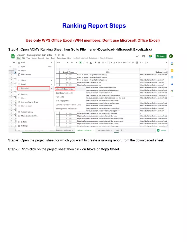
Ranking Report Steps Use only WPS Office Excel (WFH members: Don't use Microsoft Office Excel) Step-1: Open ACM’s Ranking Sheet then Go to File menu->Download->Microsoft Excel(.xlsx) Step-2: Open the project sheet for which you want to create a ranking report from the downloaded sheet. Step-3: Right-click on the project sheet then click on Move or Copy Sheet
Then select the New Workbook & select the checkbox Create a copy then press the Ok button Step-4: Select all the rows & columns by clicking on the corner then click on the Home menu -> Freeze Panes->Unfreeze Panes
Step-5: Again select all the rows & columns by clicking on the corner then right-click and press Unhide option to unhide rows & columns. Step-6: Remove unnecessary columns before the current month’s ranking column.
Step-6: Remove formulas for the positions from both Main and Extra Keywords Step-7: Remove No. column
Step-8: Select all extra keyword rows and Sort them by clicking on Data->Sort->Custom Sort Make sure your current month's ranking column should be in Column C.
Step-9: Remove the rows whose keywords positions are above 10 & Not in 100. But keep rows for Google Places. Step-10: Remove blank columns and merge Main & Extra keywords
Step-11: Now again select all keyword rows and Sort them by clicking on Data->Sort->Custom Sort Note: Make sure you have marked the checkbox My data has headers if you selected header otherwise uncheck the checkbox My data has headers. Step-12: Select the rows of the Google Places 1 keywords & press Ctrl+X key
Step-13: Select the row of the 1st position keyword and then right-click ->Insert Cut Cells (To paste the rows which we selected and Cut ) In short, we place Google Places 1 keyword above the regular 1st position keywords. Repeat this step for Google Places 2, Google Places 3 - Google Places 2 will be placed before the 2 position keywords - Google Places 3 will be placed before the 3 position keywords Step-14: Select the header row and set the Text color as Lime
Again select the header row and set the background color as Navy Press Ctrl+B to bold the header row
Step-15: Select the Search Volume column & Press Ctrl+H to replace blank columns with 0-10 and then press Replace All button. Step-16: Again select the Search Volume column to replace “K” with “000” by pressing Ctrl+H like:
Step-17: Now, select all the Columns from Column C to put Dash (-) in the blank cells. Press Ctrl+H and Keep find what as blank & fill Replace with the field as “-”
Step-18: Select all the columns from B column And set alignment as Center like:
Step-20: Select all columns and rows by clicking Corner and Selecting Middle Align to set Row text alignment in the middle. Step-21: Select all columns and rows by clicking Corner and selecting Font Type: Arial & Size: 10
Step-22: Again select all the columns and rows by clicking Corner & Double click on Any row or a column to Auto adjust rows & columns. Step-23: Make all the bold text Normal text except the Header row. Step-24: Check after the last Column & row if you see any formatting then clear them by clicking Home->Format->Clear->Formats
Step-25: Select all the Keywords and go to Data -> Highlight Duplicates Note: It will be auto adjust the range if you have selected Keywords before otherwise, you have to select a range
Step-26: Now select all of your rows & columns up to your data (Don’t select range out of your data) and give all borders to selected rows & columns. Step-27: Save your file with the name like: [Project Name without space]-Ranking-Report-[Month]-[Year] Ex. DapperEthnic-Ranking-Report-Feb-2023 Notes 1. While making Google + Bing reports every 3 months, Keep in mind the following points:
➔ Create a single spreadsheet with two sheets with the names "Google Rankings" & "Bing Rankings" ➔ To create a Bing ranking report, follow the steps same as a Google ranking report ➔ Remove Bing Rankings from the Google Rankings sheet ★ Bing ➔ Remove Google Rankings from the Bing Rankings sheet ➢ We Find only main keyword rankings up to 50 positions. ➢ Sort by the current month’s ranking as same we do for google rankings ➢ Move Bing Places rows as same as we move for Google Places. ➢ Don’t include Search Volume in the Bing Ranking report 2. Don’t hide additional rows and columns (It will increase the storage size of an excel sheet)