ABSTRACT

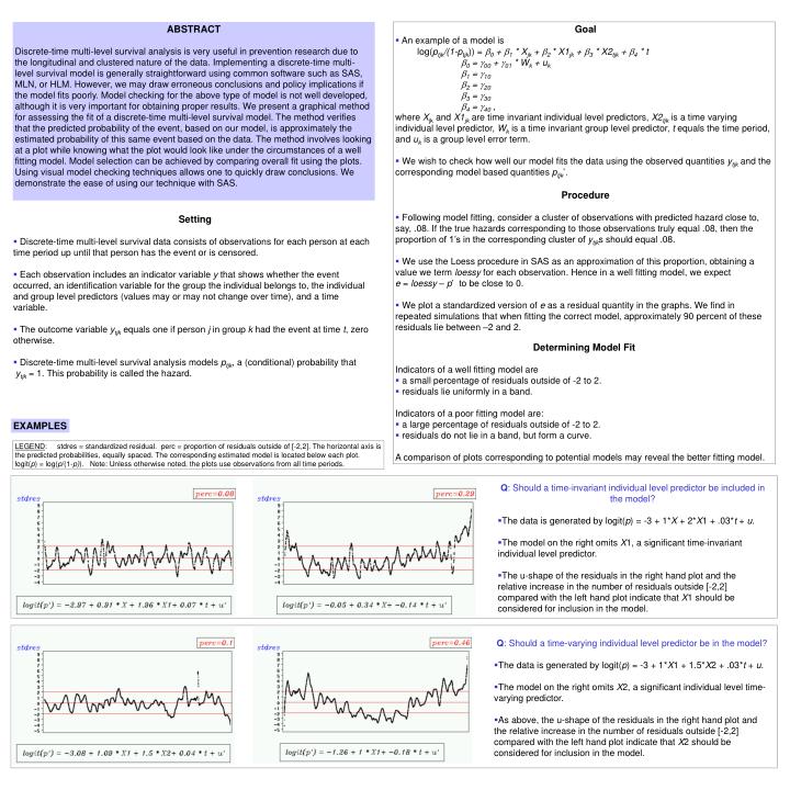
1. ABSTRACT Discrete-time multi-level survival analysis is very useful in prevention research due to the longitudinal and clustered nature of the data. Implementing a discrete-time multi-level survival model is generally straightforward using common software such as SAS, MLN, or HLM. However, we may draw erroneous conclusions and policy implications if the model fits poorly. Model checking for the above type of model is not well developed, although it is very important for obtaining proper results. We present a graphical method for assessing the fit of a discrete-time multi-level survival model. The method verifies that the predicted probability of the event, based on our model, is approximately the estimated probability of this same event based on the data. The method involves looking at a plot while knowing what the plot would look like under the circumstances of a well fitting model. Model selection can be achieved by comparing overall fit using the plots. Using visual model checking techniques allows one to quickly draw conclusions. We demonstrate the ease of using our technique with SAS. • Goal • An example of a model is • log(ptjk/(1-ptjk)) = b0 + b1 * Xjk + b2 * X1jk + b3 * X2tjk + b4 * t • b0 = g00 + g01 * Wk + uk • b1 = g10 • b2 = g20 • b3 = g30 • b4 = g40 , • where Xjk and X1jk are time invariant individual level predictors, X2tjk is a time varying individual level predictor, Wk is a time invariant group level predictor, t equals the time period, and uk is a group level error term. • We wish to check how well our model fits the data using the observed quantities ytjk and the corresponding model based quantities ptjk’. • Procedure • Following model fitting, consider a cluster of observations with predicted hazard close to, say, .08. If the true hazards corresponding to those observations truly equal .08, then the proportion of 1’s in the corresponding cluster of ytjks should equal .08. • We use the Loess procedure in SAS as an approximation of this proportion, obtaining a value we term loessy for each observation. Hence in a well fitting model, we expect e = loessy – p’to be close to 0. • We plot a standardized version of e as a residual quantity in the graphs. We find in repeated simulations that when fitting the correct model, approximately 90 percent of these residuals lie between –2 and 2. • Determining Model Fit • Indicators of a well fitting model are • a small percentage of residuals outside of -2 to 2. • residuals lie uniformly in a band. • Indicators of a poor fitting model are: • a large percentage of residuals outside of -2 to 2. • residuals do not lie in a band, but form a curve. • A comparison of plots corresponding to potential models may reveal the better fitting model. • Setting • Discrete-time multi-level survival data consists of observations for each person at each time period up until that person has the event or is censored. • Each observation includes an indicator variable y that shows whether the event occurred, an identification variable for the group the individual belongs to, the individual and group level predictors (values may or may not change over time), and a time variable. • The outcome variable ytjk equals one if person j in group k had the event at time t, zero otherwise. • Discrete-time multi-level survival analysis models ptjk, a (conditional) probability that ytjk = 1. This probability is called the hazard. EXAMPLES LEGEND: stdres = standardized residual. perc = proportion of residuals outside of [-2,2]. The horizontal axis is the predicted probabilities, equally spaced. The corresponding estimated model is located below each plot. logit(p) = log(p/(1-p)). Note: Unless otherwise noted, the plots use observations from all time periods. Q: Should a time-invariant individual level predictor be included in the model? • The data is generated by logit(p) = -3 + 1*X + 2*X1 + .03*t + u. • The model on the right omits X1, a significant time-invariant individual level predictor. • The u-shape of the residuals in the right hand plot and the relative increase in the number of residuals outside [-2,2] compared with the left hand plot indicate that X1 should be considered for inclusion in the model. Q: Should a time-varying individual level predictor be in the model? • The data is generated by logit(p) = -3 + 1*X1 + 1.5*X2 + .03*t + u. • The model on the right omits X2, a significant individual level time-varying predictor. • As above, the u-shape of the residuals in the right hand plot and the relative increase in the number of residuals outside [-2,2] compared with the left hand plot indicate that X2 should be considered for inclusion in the model.

2. Q: Should a time-invariant group level predictor be in the model? • The data is generated by logit(p) = -3 + 1*X + 1.5*W + .02*t + u. • The model on the right omits W, a significant group level time-invariant predictor. • The non-uniform shape of the residuals in the right hand plot and the large increase in number of residuals outside of [-2,2] compared with the left hand plot indicate that W should be considered for inclusion in the model. Q: Is the inclusion of a group level error term contributing to the predicted hazard? • The data is generated by logit(p) = -1 + 1*X + u. • The model on the right omits u, a group level error term. • The large increase in the number of residuals outside [-2,2] in the right hand plot suggests including the group level error term in the model. Q: What is a reasonable form for the baseline hazard? • The data is generated by logit(p) = -1 + 1*X + .4*t - .06*t*t + u. • The model on the right omits t*t, the time-squared term. • It seems that the time-squared term is important. However, it is more useful to look at plots that do not use all time periods simultaneously, as the following two plots show. • The data is the same as in the previous example. • These plots use only observations corresponding to time periods 5 and later. • The squared term is needed in the model, based on the residual plots. Linear and quadratic baseline hazards can be similar in shape for earlier time periods, but for later time periods when the true hazard is small, addition of a quadratic term is necessary to get a good fit. • CONCLUSIONS • The approach described here provides the prevention researcher with a graphical means of verifying model fit and justifying predictor inclusion based on its contribution to predicting event occurrence. • Over numerous simulated data sets, we find that the method detects significant, time-varying and time-invariant individual level predictors and group level predictors, and ascertains an accurate form for the baseline hazard. • In the case of a constant baseline hazard, omission of a group level error term can be detected. Future research will address the non-constant case. • Future work includes plots of residuals versus predictors, martingale residual plots, and the case of when all the predicted hazards very small. References Kay, R. & S. Little (1986). Assessing the Fit of the Logistic Model: A Case Study of Children with the Haemolytic Uraemic Syndrome. Applied Statistics, 36, 16-30. Barber, J.S., S.A. Murphy, W.G. Axinn, & J. Maples (2000). Discrete-time Multilevel Survival Analysis. Sociological Methodology, 30, 201-235. This research was supported by the National Institute on Drug Abuse Grant # 2 P50 DA10075