Download

1 / 69
700 likes | 946 Views
Recap. Last weekTheoretical Development of Capital Assets Pricing ModelDistortion of vN

E N D
1. Behavioural Finance Lecture 04
Actual Finance Markets Behaviour
2. Recap Last week
Theoretical Development of Capital Assets Pricing Model
Distortion of vN&M�s Expected Utility Analysis
Why �Maximising Expected Return� is not rational
This week
How the data destroyed CAPM
3. Overview CAPM assumes financial markets �efficient�
If so, prices follow a �random walk�
Deviations from trend follow Normal distribution
Change of huge change (+ or � 5 Standard deviations) vanishingly rare
Actual data shows huge changes extremely common
So markets not �efficient� in economists sense
Might still be �efficient� in common sense�fast trades, rapid assimilation of data
But key data might include what other traders do or believe
Feedback causes extreme nonlinearities, booms and busts�
4. CAPM and Market �Efficiency� CAPM became part of �Efficient Markets Hypothesis� (EMH)
Model in which prices set in equilibrium process
Explanation of why traders couldn�t profit by exploiting mis-pricing in market
Share prices accurately reflect all available information
No mis-pricing to exploit
Alternative view possible
Markets �chaotic�
Prices set in disequilibrium process
Information on mis-pricing exists
but (generally) too complicated to work it out�
5. Chaos or Efficiency? Systems with strong nonlinear feedbacks won�t be �efficient� as economists use the word
meaning �values remain close to equilibrium�
But will be impossible to predict
Similar to �traders can�t exploit market mis-pricing� component of EMH
Instead, nonlinear systems operate far from equilibrium
If stock market behaves this way, can be unpredictable even if prices far from equilibrium
�Mis-pricing� can exist
But be too difficult to exploit
An example� Lorenz�s weather model
6. Lorenz�s Butterfly Model of fluid flow caused by heat
Convection in fluid
rising and falling columns of fluid
causing turbulence, storms
E.g., columns of rising & falling magma in earth�s core
7. Lorenz�s Butterfly Intensity of convection (x)
Temperature gap between rising & falling current (y)
Deviation of Temperature profile from linear (z)
8. Lorenz�s Butterfly To find equilibrium, set all 3 rates of change to zero:
9. Lorenz�s Butterfly So there are 3 solutions:
x=y=z=0
10. Lorenz�s Butterfly How does system behave?
Can show (with matrix mathematics) that
For some values of parameters
All 3 equilibia are unstable!
So how to know how the system will behave?
Let�s simulate it�
Many programs exist to simulate dynamic models
More on these later, but the basic idea
Represent system as
Flowchart; or
Set of equations
Iterate from starting position
see what happens over time�
11. Lorenz�s Butterfly The basic idea is:
Take a variable (e.g., population)
Multiply its current value by its growth rate
Integrate this flow
�Add� the increments to population to current population
Add to initial population�
Estimate future population
12. Lorenz�s Butterfly Lorenz�s model looks like this in Vissim:
13. Lorenz�s Butterfly So the system is never in equilibrium; and
Follows complex cycles that are
Unpredictable
A-periodic (no set period as for sin, cosine etc.)
But have �hidden� structure behind the �chaos�:
14. Stock Markets and Chaos? Beniot Mandelbrot thought so�
(more on him and chaos soon�)
IF stock markets were �efficient� in CAPM sense
Prices �reflect all available information�
Accurately value future earnings of companies
(given what is known now)
THEN prices should follow �random walk with drift�
�Random walk� because of random arrival of news
News varies estimates of future earnings
�Drift� because prices tend upwards over time
Since news (�shocks� from non-economic systems) arrives at random, stock prices should move randomly
Basic pattern should be �Gaussian�:
15. Random walking� �Gaussian� distributions result from random processes
Toss of a coin, roll of 2 dice, roulette wheel spin�
In the limit�
Do them often enough and�
Outcome will be fully described by
Average outcome
Toss ten coins, average 5 heads, 5 tails;
Roll of 2 dice, average 7
And standard deviation
68% within +/- 1 standard deviations
95% within +/- 2 standard deviations�
16. Random walking� E.g., height of American males�
Average 178cm
Standard deviation 8cm
Roughly 150 million of them
So height distribution should (& does) look like this:
17. Random walking� Tiny insignificant fraction
Taller than 2 metres
(2.75 standard deviations above mean)
Shorter than 160cm
2.25 standard deviations below)
18. Random walking� If the stock market was following a random walk, then it would look the same:
Average daily movement
Standard deviation
68% within +/- 1 standard deviations
95% within +/- 2 standard deviations�
Dow Jones from 1914-2009
Average daily movement 0.027%
Standard deviation 1.136%
24,437 trading days (till August 15 2009)
So the market �should� look like this�
19. Random walking� Simulated data�
20. Random walking down Wall Street� Same pattern as for height of Americans�
21. An actual walk down Wall Street� Similar pattern it seems, but�
Many more events near average movement
�Tail� (large negative or positive movements) clearly longer
22. An actual walk down Wall Street� Whoops�
23. An actual walk down Wall Street� Many more large negative movements than positive in actual data
Let�s re-rank data from smallest to biggest movement and see what we get�
24. An actual walk down Wall Street� Both data series have the same number of points
24,436 trading days from 1914-2009
�Random walk� simulation predicts much narrower range of daily movements in stock prices
25. An actual walk down Wall Street� EMH drastically underestimates volatility of market:
26. Random or Fractal Walk Down Wall Street?� EMH/CAPM argued returns can�t be predicted
Random walk/Martingale/Sub-martingale
Distribution of returns should be �Gaussian�
Non-EMH theories (Fractal Markets, etc.) argue distribution should be non-random
Basic characteristics of fractal distributions
�Fat tails��many more extreme events than random distribution
Extreme events of any magnitude possible vs vanishingly unlikely for random
Random: Odds of 5% fall of DJIA? Less than 2 in a million� (biggest fall in simulated data 4.467%)
How many years needed to see one 5% fall?
27. Random or Fractal Walk Down Wall Street?� Power law distribution very different to Gaussian:
Number of size X events ? X raised to some power
28. Random or Fractal Walk Down Wall Street?� Power law fit Dow Jones:
29. Random or Fractal Walk Down Wall Street?� You betcha!
30. Random or Fractal Walk Down Wall Street?� Belief system is
in equilibrium
changes due to random shocks
Results in prediction that huge events vanishingly rare
Actual data manifestly different:
31. Random or Fractal Walk Down Wall Street?�
32. Random or Fractal Walk Down Wall Street?�
33. Random or Fractal Walk Down Wall Street?�
34. Random or Fractal Walk Down Wall Street?� Data clearly not random
More sophisticated analyses (future lecture) confirm this
Underlying process behind stock market therefore
Partly deterministic
Highly nonlinear
Interacting �Bulls� & �Bears�
Underlying economic-financial feedbacks
Economics needs
a theory of endogenous money�
A theory of nonlinear, nonequilibrium finance�
Why do most economists still cling to the EMH?
35. CAPM: The original belief CAPM fitted belief in equilibrium behaviour of finance markets, but required extreme assumptions of:
�a common pure rate of interest, with all investors able to borrow or lend funds on equal terms. Second, we assume homogeneity of investor expectations: investors are assumed to agree on the prospects of various investments the expected values, standard deviations and correlation coefficients�
Justified on basis of methodology and agreement with theory:
�Needless to say, these are highly restrictive and undoubtedly unrealistic assumptions. However, since the proper test of a theory is not the realism of its assumptions but the acceptability of its implications, and since these assumptions imply equilibrium conditions which form a major part of classical financial doctrine, it is far from clear that this formulation should be rejected-especially in view of the dearth of alternative models leading to similar results.� (Sharpe 1964: 433-434)
Fama (1969) applied �the proper test� and hit paydirt�
36. Fama 1969: Data supports the theory �For the purposes of most investors the efficient markets model seems a good first (and second) approximation to reality. In short, the evidence in support of the efficient markets model is extensive, and (somewhat uniquely in economics) contradictory evidence is sparse.� (Fama 1969: 436)
Fama�s paper reviewed analyses of stock market data up till 1966�
Table 1, 1957-66; Ball & Brown 1946-66; Jensen 1955-64;
Remember longer term look at the DJIA data?...
37. The CAPM: Evidence Fit shows average exponential growth 1915-1999:
index well above or below except for 1955-1973
38. The Capital Assets Pricing Model Remember Sharpe�s assumptions?:
�a common pure rate of interest, with all investors able to borrow or lend funds on equal terms�
homogeneity of investor expectations: investors are assumed to agree on the prospects of various investments.
And his defence of them?
�Needless to say, these are highly restrictive and undoubtedly unrealistic assumptions. However, since the proper test of a theory is not the realism of its assumptions but the acceptability of its implications��
How valid is this defence?
39. The �Instrumental� Defence Appeal to Milton Friedman�s �Methodology of Positive Economics�:
�Realism� of assumptions irrelevant:
�the more significant the theory, the more unrealistic the assumptions� a hypothesis is important if it �explains� much by little� (Friedman 1953: pp. 14-15)
Sharpe invokes Friedman�s �Instrumental� Defence:
OK to assume investors agree on future prospects of all shares, etc., even if not true�
So long as resulting model fits the data???
(See History of Economic Thought Methodology lecture), but in summary)
Instrumental defence false�
40. The �Instrumental� Defence Logical consistency of assumptions can be challenged, not just realism
�Proof by contradiction� also
can�t assume �square root of 2 is rational�;
likewise can�t assume �all investors identical� to �aggregate�
Sciences do attempt to build theories which are essentially descriptions of reality
Musgrave (1981) argues Friedman�s �significant theory, unrealistic assumptions� position invalid
Classifies assumptions into 3 classes
Negligibility assumptions
Domain Assumptions
Heuristic Assumptions
41. Within Economics: Instrumentalism Negligibility Assumptions
Assert that some factor is of little or no importance in a given situation
e.g., Galileo�s experiment to prove that weight does not affect speed at which objects fall
dropped two different size lead balls from Leaning Tower of Pisa
�assumed� (correctly) air resistance �negligible� at that altitude for dense objects, therefore ignored air resistance
Domain assumptions
Assert that theory is relevant if some assumed condition applies, irrelevant if condition does not apply
42. Within Economics: Instrumentalism e.g., Newton�s theory of planetary motion �assumed� there was only one planet
if true, planet follows elliptical orbit around sun.
if false & planets relatively massive, motion unpredictable. Poincare (1899) showed
there was no formula to describe paths
paths were in fact �chaotic�
planets in multi-planet systems therefore collide
present planets evolved from collisions
�evolutionary� explanation for present-day
roughly elliptical orbits
absence of collisions between planets
43. Classes of assumptions Heuristic
assumption known to be false, but used as stepping stone to more valid theory
e.g., in developing theory of relativity, Einstein assumes that distance covered by person walking across a train carriage equals trigonometric sum of
forward movement of train
sideways movement of passenger
44. Just where are markets efficient? The Efficient Markets Hypothesis: assume
All investors have identical accurate expectations of future
All investors have equal access to limitless credit
Negligible, Domain or Heuristic assumptions?
Negligible? No: if drop them, then according to Sharpe �The theory is in a shambles� (see last lecture)
Heuristic? No, EMH was �end of the line� for Sharpe�s logic: no subsequent theory developed which
replaced risk with uncertainty, or
took account of differing inaccurate assumptions, different access to credit, etc.
Basis of eventual empirical failure of CAPM
45. The CAPM: Evidence Sharpe�s qualms ignored & CAPM takes over economic theory of finance
Initial evidence seemed to favour CAPM
Essential ideas:
Price of shares accurately reflects future earnings
With some error/volatility
Shares with higher returns more strongly correlated to economic cycle
Higher return necessarily paired with higher volatility
Investors simply chose risk/return trade-off that suited their preferences
Initial research found expected (positive) relation between return and degree of volatility
But were these results a fluke?
46. The CAPM: Evidence Sharpe�s CAPM paper published 1964
Initial CAPM empirical research on period 1950-1960�s
As noted in last lecture
Dow Jones advance steadily from 1949-1965
July 19 1949 DJIA cracks 175
Feb 9 1966 DJIA sits on verge of 1000 (995.15)
467% increase over 17 years
Continued for 2 years after Sharpe�s paper
Then period of near stagnant stock prices
Fama�s enthusiastic empirical paper on CAPM used data from 1950-1966:
47. The CAPM: Evidence According to Fama 1969 Evidence supports the CAPM
�This paper reviews the theoretical and empirical literature on the efficient markets model� We shall conclude that, with but a few exceptions, the efficient markets model stands up well.� (383)
Assumptions unrealistic but that doesn�t matter:
�the results of tests based on this assumption depend to some extent on its validity as well as on the efficiency of the market. But some such assumption is the unavoidable price one must pay to give the theory of efficient markets empirical content.� (384)
48. The CAPM: Evidence According to Fama 1969 CAPM good guide to market behaviour
�For the purposes of most investors the efficient markets model seems a good first (and second) approximation to reality.� (416)
Results conclusive
�In short, the evidence in support of the efficient markets model is extensive, and (somewhat uniquely in economics) contradictory evidence is sparse.� (416)
Just one anomaly admitted to
Large movements one day often followed by large movements the next��volatility clustering��
49. The CAPM: Evidence According to Fama 1969 �one departure from the pure independence assumption of the random walk model has been noted �
large daily price changes tend to be followed by large daily changes.
The signs of the successor changes are apparently random, however, which indicates that the phenomenon represents a denial of the random walk model but not of the market efficiency hypothesis�
But since the evidence indicates that the price changes on days following the initial large change are random in sign,
the initial large change at least represents an unbiased adjustment to the ultimate price effects of the information, and this is sufficient for the expected return efficient markets model.� (396)
50. The CAPM: Evidence 50-66 and 1914-2009 But was this �evidence� just a fluke?
Result from considering too narrow a range of data?
Dow Jones 1950-1966:
51. The CAPM: Evidence 50-66 and 1914-2009 What about volatility?
Daily movements 50-66:
52. The CAPM: Evidence 50-66 and 1914-2009 Superimposing �EMH� simulated data to actual
1950-66
53. The CAPM: Evidence 50-66 and 1914-2009 Daily movement indicator looks OK for 50-66 too:
1950-66 data:
54. The CAPM: Evidence 50-66 and 1914-2009 Large movements data looks OK vs simulated data:
Actual 1950-66
55. The CAPM: Evidence 50-66 and 1914-2009 Far more large movements in data than simulation:
Actual 14-09:
56. The CAPM: Evidence 50-66 and 1914-2009 So early �success� of CAPM a statistical aberration
Period used
Too short
Just 16 years data when 60 years available
Too stable
50-66 period of low debt, high financial resilience, low speculation
Versus 14-09 period including 4 major market crashes: 29, 87, 2000, 2008
Fama forced to admit empirical defeat of CAPM in 2004:
(But should have been rejected on scientific methodology grounds in the first place!)
57. The CAPM: Evidence According to Fama 2004 �The attraction of the CAPM is that it offers powerful and intuitively pleasing predictions about how to measure risk and the relation between expected return and risk.
Unfortunately, the empirical record of the model is poor�poor enough to invalidate the way it is used in applications.
The CAPM's empirical problems may reflect theoretical failings, the result of many simplifying assumptions�
In the end, we argue that whether the model's problems reflect weaknesses in the theory or in its empirical implementation, the failure of the CAPM in empirical tests implies that most applications of the model are invalid.� (Fama & French 2004: 25)
58. The CAPM: Evidence According to F&F 2004 Clearly admits assumptions dangerously unrealistic:
�The first assumption is complete agreement given market clearing asset prices at t-1, investors agree on the joint distribution of asset returns from t-1 to t.
And this distribution is the true one�that is, it is the distribution from which the returns we use to test the model are drawn. The second assumption is that there is borrowing and lending at a risk free rate, which is the same for all investors and does not depend on the amount borrowed or lent.� (26)
Bold emphasis: model assumes all investors know the future
Assumptions, which once �didn�t matter� (see Sharpe earlier) are now crucial�
59. The CAPM: Evidence According to F&F 2004 �The assumption that short selling is unrestricted is as unrealistic as unrestricted risk-free borrowing and lending�
But when there is no short selling of risky assets and no risk-free asset, the algebra of portfolio efficiency says that portfolios made up of efficient portfolios are not typically efficient.
This means that the market portfolio, which is a portfolio of the efficient portfolios chosen by investors, is not typically efficient. And the CAPM relation between expected return and market beta is lost.� (32)
Still some hope that, despite lack of realism, data might save the model�
60. The CAPM: Evidence According to F&F 2004 �The efficiency of the market portfolio is based on many unrealistic assumptions, including complete agreement and either unrestricted risk-free borrowing and lending or unrestricted short selling of risky assets. But all interesting models involve unrealistic simplifications, which is why they must be tested against data.� (32)
Unfortunately, no such luck�
40 years of data strongly contradict all versions of CAPM
Returns not related to betas
Other variables (book to market ratios etc.) matter
Linear regressions on data differ strongly from risk free rate (intercept) & beta (slope) calculations from CAPM
61. The CAPM: Evidence According to F&F 2004 Tests of the CAPM are based on three implications�
�First, expected returns on all assets are linearly related to their betas, and no other variable has marginal explanatory power.
Second, the beta premium is positive, meaning that the expected return on the market portfolio exceeds the expected return on assets whose returns are uncorrelated with the market return.
Third, � assets uncorrelated with the market have expected returns equal to the risk-free interest rate, and the beta premium is the expected market return minus the risk-free rate.� (32)
62. The CAPM: Evidence According to F&F 2004 �There is a positive relation between beta and average return, but it is too "flat." � the Sharpe-Lintner model predicts that
the intercept is the risk free rate and
the coefficient on beta is the expected market return in excess of the risk-free rate, E(RM) - R.
The regressions consistently find that the intercept is greater than the average risk-free rate�, and the coefficient on beta is less than the average excess market return� (32)
63. The CAPM: Evidence According to F&F 2004 Average Annualized Monthly Return versus Beta for Value Weight Portfolios Formed on Prior Beta, 1928-2003
64. The CAPM: Evidence According to F&F 2004 The hypothesis that market betas completely explain expected returns �
Starting in the late 1970s� evidence mounts that much of the variation in expected return is unrelated to market beta�� (34)
Fama and French (1992) update and synthesize the evidence on the empirical failures of the CAPM�
they confirm that size, earnings-price, debt equity and book-to-market ratios add to the explanation of expected stock returns provided by market beta.� (36)
Best example of failure of CAPM as guide to building investment portfolios:
Book to Market (B/M) ratios provide far better guide than Beta�
65. The CAPM: Evidence According to F&F 2004 �Average returns on the B/M portfolios increase almost monotonically, from 10.1 percent per year for the lowest B/M group to an impressive 16.7 percent for the highest.
But the positive relation between beta and average return predicted by the CAPM is notably absent�
the portfolio with the lowest book-to-market ratio has the highest beta but the lowest average return.
The estimated beta for the portfolio with the highest book-to�market ratio and the highest average return is only 0.98. With an average annualized value of the riskfree interest rate, Rf, of 5.8 percent and an average annualized market premium, Rm - Rf, of 11.3 percent,
the Sharpe-Lintner CAPM predicts an average return of 11.8 percent for the lowest B/M portfolio and 11.2 percent for the highest, far from the observed values, 10.1 and 16.7 percent.�
66. The CAPM: Evidence According to F&F 2004 Average Annualized Monthly Return versus Beta for Value Weight Portfolios Formed on B/M, 1963-2003
67. The CAPM: Evidence According to F&F 2004 End result: CAPM should not be used.
�The � CAPM � has never been an empirical success� The problems are serious enough to invalidate most applications of the CAPM.
For example, finance textbooks often recommend using the � CAPM risk-return relation to estimate the cost of equity capital� [But] CAPM estimates of the cost of equity for high beta stocks are too high � and estimates for low beta stocks are too low�
The CAPM � is nevertheless a theoretical tour de force. We continue to teach the CAPM as an introduction to the fundamental concepts of portfolio theory and asset pricing�
But we also warn students that despite its seductive simplicity, the CAPM's empirical problems probably invalidate its use in applications.� (F&F 2004: 46-47)
68. Fama & French 2004: Data kills the theory �The attraction of the CAPM is that it offers powerful and intuitively pleasing predictions about how to measure risk and the relation between expected return and risk.
Unfortunately, the empirical record of the model is poor�poor enough to invalidate the way it is used in applications.� (Fama & French 2004: 25)
69. Random or Fractal Walk Down Wall Street?� Many don�t know that developers of CAPM have abandoned it
Most don�t know that any alternative exists, so teach what they know
But alternatives do exist
�Fractal/Coherent/Inefficient� Markets in finance
In Economics?
Key aspect of CAPM:
How investments are financed doesn�t affect value of firm (determined solely by net present value of investments�)
As a result, finance doesn�t affect economics
So since CAPM is false, finance does affect economics�