Download
1 / 56
580 likes | 917 Views
Chapter 7 Generating and Processing Random Signals. 第一組 電機四 B93902016 蔡馭理 資工四 B93902076 林宜鴻. Outline. Outline. Stationary and Ergodic Process Uniform Random Number Generator Mapping Uniform RVs to an Arbitrary pdf Generating Uncorrelated Gaussian RV Generating correlated Gaussian RV

E N D
Chapter 7Generating and Processing Random Signals 第一組 電機四 B93902016蔡馭理 資工四 B93902076林宜鴻
Outline Outline • Stationary and Ergodic Process • Uniform Random Number Generator • Mapping Uniform RVs to an Arbitrary pdf • Generating Uncorrelated Gaussian RV • Generating correlated Gaussian RV • PN Sequence Generators • Signal processing
Random Number Generator • Noise, interference • Random Number Generator- computational or physical device designed to generate a sequence of numbers or symbols that lack any pattern, i.e. appear random, pseudo-random sequence • MATLAB - rand(m,n) , randn(m,n)
Stationary and Ergodic Process • strict-sense stationary (SSS) • wide-sense stationary (WSS) Gaussian • SSS =>WSS ; WSS=>SSS • Time average v.s ensemble average • The ergodicity requirement is that the ensemble average coincide with the time average • Sample function generated to represent signals, noise, interference should be ergodic
Time average ensemble average Time average v.s ensemble average
Uniform Random Number Genrator • Generate a random variable that is uniformly distributed on the interval (0,1) • Generate a sequence of numbers (integer) between 0 and M and the divide each element of the sequence by M • The most common technique is linear congruence genrator (LCG)
Linear Congruence • LCG is defined by the operation: xi+1=[axi+c]mod(m) • x0 is seed number of the generator • a, c, m, x0 are integer • Desirable property- full period
Technique A: The Mixed Congruence Algorithm • The mixed linear algorithm takes the form: xi+1=[axi+c]mod(m) - c≠0 and relative prime tom - a-1 is a multiple of p, where p is the prime factors of m - a-1 is a multiple of 4 ifm is a multiple of 4
Example 7.4 • m=5000=(23)(54) • c=(33)(72)=1323 • a-1=k1‧2 or k2‧5 or 4‧k3 so, a-1=4‧2‧5‧k =40k • With k=6, we have a=241 xi+1=[241xi+ 1323]mod(5000) • We can verify the period is 5000, so it’s full period
Technique B: The Multiplication Algorithm With Prime Modulus • The multiplicative generator defined as : xi+1=[axi]mod(m) - m isprime (usaually large) - a is a primitive elementmod(m) am-1/m = k =interger ai-1/m ≠ k, i=1, 2, 3,…, m-2
Technique C: The Multiplication Algorithm With Nonprime Modulus • The most important case of this generator having m equal to a power of two : xi+1=[axi]mod(2n) • The maximum period is 2n/4= 2n-2 the period is achieved if - The multiplier a is 3 or 5 - The seed x0is odd
Example of Multiplication Algorithm With Nonprime Modulus a=3 c=0 m=16 x0=1
Testing Random Number Generator • Chi-square test, spectral test…… • Testing the randomness of a given sequence • Scatterplots- a plot of xi+1 as a function of xi • Durbin-Watson Test -
ScatterplotsExample 7.5 (i)rand(1,2048) (ii)xi+1=[65xi+1]mod(2048) (iii)xi+1=[1229xi+1]mod(2048)
Durbin-Watson Test (1) Let X = X[n] & Y = X[n-1] Assume X[n] and X[n-1] are correlated and X[n] is an ergodic process Let
Durbin-Watson Test (2) X and Z are uncorrelated and zero mean D>2 – negative correlation D=2 –-uncorrelation (most desired) D<2 – positive correlation
Example 7.6 • rand(1,2048) - The value of D is 2.0081 and ρ is 0.0041. • xi+1=[65xi+1]mod(2048) - The value of D is 1.9925 and ρ is 0.0037273. • xi+1=[1229xi+1]mod(2048) - The value of D is 1.6037 and ρ is 0.19814.
Minimum Standards • Full period • Passes all applicable statistical tests for randomness. • Easily transportable from one computer to another • Lewis, Goodman, and Miller Minimum Standard (prior to MATLAB 5) xi+1=[16807xi]mod(231-1)
Mapping Uniform RVs to an Arbitrary pdf • The cumulative distribution for the target random variable is known in closed form – Inverse Transform Method • The pdf of target random variable is known in closed form but the CDF is not known in closed form – Rejection Method • Neither the pdf nor CDF are known in closed form – Histogram Method
Inverse Transform Method • CDF FX(X) are known in closed form • U = FX (X) = Pr { X≦ x } X = FX-1(U) • FX (X) = Pr { FX-1(U) ≦ x } = Pr {U≦ FX (x) }= FX (x)
Example 7.8 (1) • Rayleigh random variable with pdf – ∴ Setting FR(R) = U
Example 7.8 (2) ∵RV 1-U is equivalent to U (have same pdf) ∴ Solving for R gives • [n,xout] = hist(Y,nbins) - • bar(xout,n) - plot the histogram
The Histogram Method • CDF andpdf are unknown • Pi =Pr{xi-1 < x < xi} = ci(xi-xi-1) • FX(x) = Fi-1 + ci(xi-xi-1) • FX(X) = U = Fi-1 + ci(X-xi) more samples more accuracy!
Rejection Methods (1) • Having a targetpdf • MgX(x)≧ fX(x), all x
Rejection Methods (2) • Generate U1 and U2 uniform in (0,1) • Generate V1 uniform in (0,a), where a is the maximum value of X • Generate V2 uniform in (0,b), where b is at least the maximum value of fX(x) • If V2≦ fX(V1), set X= V1. If the inequality is not satisfied, V1 and V2 are discarded and the process is repeated from step 1
Generating Uncorrelated Gaussian RV • Its CDF can’t be written in closed form,so Inverse method can’t be used and rejection method are not efficient • Other techniques 1.The sum of uniform method 2.Mapping a Rayleigh to Gaussian RV 3.The polar method
The Sum of Uniforms Method(1) • 1.Central limit theorem • 2.See next . • 3. represent independent uniform R.V is a constant that decides the var of Y converges to a Gaussian R.V.
The Sum of Uniforms Method(2) • Expectation and Variance • We can set to any desired value • Nonzero at
The Sum of Uniforms Method(3) • Approximate Gaussian • Maybe not a realistic situation.
Mapping a Rayleigh to Gaussian RV(1) • Rayleigh can be generated by U is the uniform RV in [0,1] • Assume X and Y are indep. Gaussian RV and their joint pdf
Mapping a Rayleigh to Gaussian RV(2) • Transform let and and
Mapping a Rayleigh to Gaussian RV(3) • Examine the marginal pdf R is Rayleigh RV and is uniform RV
The Polar Method • From previous • We may transform
The Polar Method Alothgrithm • 1.Generate two uniform RV, and and they are all on the interval (0,1) • 2.Let and ,so they are independent and uniform on (-1,1) • 3.Let if continue, else back to step2 • 4.Form • 5.Set and
Establishing a Given Correlation Coefficient(1) • Assume two Gaussian RV X and Y ,they are zero mean and uncorrelated • Define a new RV • We also can see Z is Gaussian RV • Show is correlation coefficient relating X and Z
Establishing a Given Correlation Coefficient(2) • Mean,Variance,Correlation coefficient
Establishing a Given Correlation Coefficient(3) • Covariance between X and Z • as desired
Pseudonoise(PN) Sequence Genarators • PN generator produces periodic sequence that appears to be random • Generated by algorithm using initial seed • Although not random,but can pass many tests of randomness • Unless algorithm and seed are known,the sequence is impractical to predict
Property of Linear Feedback Shift Register(LFSR) • Nearly random with long period • May have max period • If output satisfy period ,is called max-length sequence or m-sequence • We define generator polynomial as • The coefficient to generate m-sequence can always be found
Property of m-sequence • Has ones, zeros • The periodic autocorrelation of a m-sequence is • If PN has a large period,autocorrelation function approaches an impulse,and PSD is approximately white as desired
Signal Processing • Relationship 1.mean of input and output 2.variance of input and output 3.input-output cross-correlation 4.autocorrelation and PSD