Understanding Binomial Distributions: Predictions and Applications

1. Binomial Distributions Chapter 5.3 – Probability Distributions and Predictions Mathematics of Data Management (Nelson) MDM 4U Authors: Gary Greer (with K. Myers)

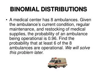
2. Our Problem… • suppose students either like math or they don’t • suppose 5% of students like math • if you had 300 students, how likely would it be that 20 of them liked math? • this can be modeled as a binomial distribution • in statistics it is important in looking at how likely a situation is to have occurred randomly • if it is very unlikely to have occurred, it lends support to the significance of a finding

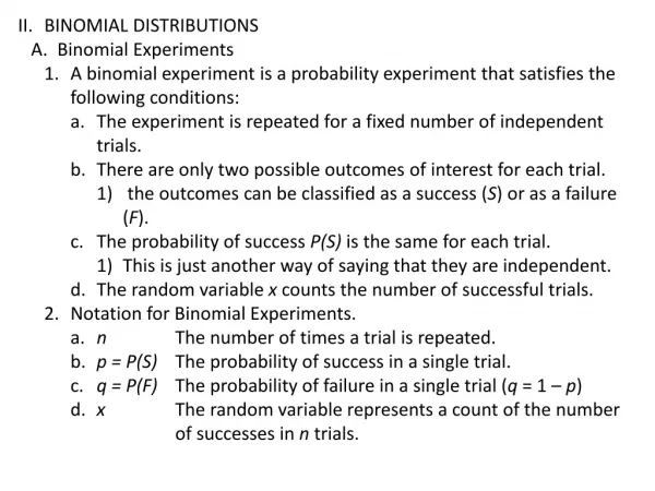
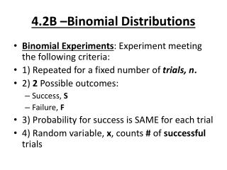
3. Binomial Experiments • a binomial experiment is any experiment that has the following properties: • there are n identical trials • there are two possible outcomes for each trial, termed success and failure • the probability of success is p and the probability of failure is 1-p • the probabilities remain constant from trial to trial • the trials are independent • repeated trials which are independent and have 2 possible outcomes (success/failure) are called Bernoulli Trials

4. Bernoulli? • Jakob Bernoulli (Basel, December 27, 1654 - August 16, 1705) • Swiss Mathematician • one of the great names in probability theory • one of a family of great minds in a variety of subjects

5. Binomial Distributions • in a binomial experiment the number of successes in n repeated Bernoulli Trials is a discrete random variable (usually called X) • X is termed a binomial random variable and its probability distribution is called a binomial distribution • the following formula provides a method of solving highly complex situations involving probability

6. Binomial Probability Distribution • consider a binomial experiment in which there are n Bernoulli trials, each with a probability of success of p • the probability of k successes in the n trials is given by:

7. Example 1 • Consider a game where a coin is flipped 5 times. You win the game if you get exactly 3 heads. What is the probability of winning? • we will let heads be a success • n = 5 • p = ½ • k = 3

8. Example 1 continued • suppose the game is changed so that you win if you get at least 3 heads • what is the probability of winning now?

9. The Batting Example • the Expected Value of a binomial experiment that consists of n Bernoulli trials with a probability of success, p, on each trial is • E(X) = n(p) • Example: Consider a baseball player who has a batting average of 0.292 • this means that his probability of getting a hit each time he is at bat is 0.292 • let a hit be a success where p = 0.292

10. a. What is the probability of no hits in the next 5 at bats?

11. b. What is the probability of 2 hits in the next 8 at bats?

12. c. What is the probability of at least 1 hit in the next 10 at bats?

13. d. What is the expected number of hits in the next 10 at bats? • E(X) = n(p) • E(X) = (10)(0.292) • = 2.92 → 3 • therefore the player can expect to get 3 hits in the next 10 at bats

14. Exercises / Homework • Homework: • page 299 #1, 3, 7, 8, 9, 10, 11, 12

15. Normal Approximation of the Binomial Distribution Chapter 5.4 – Probability Distributions and Predictions Mathematics of Data Management (Nelson) MDM 4U Authors: Gary Greer (with K. Myers)

16. Recall… • the probability of k successes in n trials (where p is the probability of success) is • this formula can only be used if we have a binomial distribution: • each trial is identical • the outcomes are either success or failure

17. This calculation is easy in simple cases… • find the probability of 30 heads in 50 trials • so there is about a 4.2% chance • however, if we wanted to find out the probability of tossing between 20 and 30 heads in 50 trial, we would need to perform at least 10 of these calculations • there is an easier way however

18. Graphing the Binomial Distribution • If the distribution is normal, we can solve complex problems in the same way we did in the last chapter • the question is: is the binomial distribution a normal one? • it turns out that if the number of trials is relatively large, the binomial distribution approximates a normal curve

19. What does it look like? • when graphed the distribution of probabilities of head looks like this • what will the mean be? • what will the standard deviation be?

20. So how do we work with all this • it turns out that a binomial distribution can be approximated by a normal distribution if: • n(p) > 5 and n(1 – p) > 5 • if this is the case, the distribution is approximated by the normal distribution

21. But doesn’t a normal curve represent continuous data and a binomial distribution represent discrete data? • Yes! • so to use a normal approximation we have to consider a range of values rather than specific discrete values • for example the range of continuous values between 4.5 and 5.5 can be represented by the discrete value 5

22. Example 1 • Tossing a coin 50 times, what is the probability that you will get tails less than 20 times • let success be tails, so n = 50 and p = 0.5 • now we can find the mean and the standard deviation

23. Example 1 continued • we will consider 0-19.5 (values below 20) times, and use it to calculate a z-score • z = 19.5 – 25 = -1.55 • 3.54 • therefore P(X < 19.5) = P(z < -1.55) • = 0.0606 • there is a 6% chance of less than 20 tails in 50 attempts

24. In terms of the normal curve, it looks like this • all the values less than 19.5 are found in the shaded area 19.5 25.0

25. Example 2 • Two dice are rolled and the sum recorded 40 times. What is the probability that a sum greater than 6 occurs in at least half of the trials? • let p be the probability of getting a sum greater than 6 • p = 6/36 + 5/36 + 4/36 + 3/36 + 2/36 + 1/36 • p = 7/12 • now we can do some calculations

26. Example 2 continued • the probability of getting a sum greater than 6 on at least half of the trials is 82%

27. Example 3 • you have a drawer with one blue mitten, one red mitten, one pink mitten and one green mitten • if you closed your eyes and picked a mitten at random 200 times (with replacement) what is the probability of choosing the pink mitten between 50 and 60 times? • so, success is considered to be drawing a pink mitten, with n = 200 and p = 0.25

28. Example 3 Continued • check to see whether the normal approximation can be used • np = 200(0.25) = 50 • n(1 – p) = 200(0.75) = 150 • since both of these are greater than 5 the binomial distribution can be approximated by the normal curve • now find the mean and standard deviation

29. Example 3 Continued • the probability of having between 50 and 60 pink mittens drawn is 0.9564 – 0.4681 = 0.4883 or about 49%

30. Exercises / Homework • Read the example on page 310 • do Page 311 # 4-10