Download
1 / 59
590 likes | 762 Views
Combining with phylogeny. Wafa Jobran Seminar in Bioinformatics Technion spring 2005. Schedule. Genome representation. GNT model. Distance based methods. True evolutionary distance. BP and IEBP variance INV and EDE variance simulation. Representing a chromosome.

E N D
Combining with phylogeny Wafa Jobran Seminar in Bioinformatics Technion spring 2005
Schedule • Genome representation. • GNT model. • Distance based methods. • True evolutionary distance. • BP and IEBP variance • INV and EDE variance • simulation.
Representing a chromosome • Chromosomeis represented byan ordering (linear or circular) of signed genes. • We assign a number to the same gene in each genome. • In the linear genome the sign indicates which strand the gene is located on. • In the circular genome we break off the circle between two neighboring genes and choosing the clockwise or counter clockwise as the positive direction.
Representing a chromosome.example: • Some of the linear representations for this genome : (1,2,3) , (2,3,1) or (-1,-3,-2)
The generalized Nadeau-Taylor model:”GNT” • We are particularly interested in the following three types of rearrangements along the edges: 1.inversions.
Inversions: starting with genome G=(g1,g2,……………………..,gn) an inversion between indices a and b, 1≤a<b≤n+1,produces: (g1,g2,…,ga-1,-gb,…,-ga,gb+1,…,gn)
The generalized Nadeau-Taylor model:”GNT” • We are particularly interested in the following three types of rearrangements along the edges: 1.inversions. 2.transposition.
Transpositions: starting with genome G=(g1, g2,……………………..,gn) a transposition on the three indices a,b,c with 1≤a<b≤n and 2≤c≤n+1,c≠a and c≠b. produces: (g1,…,ga-1,gb+1,…,gc,ga,ga+1,…,gb,gc+1,…,gn).
The generalized Nadeau-Taylor model:”GNT” • We are particularly interested in the following three types of rearrangements along the edges: 1.inversions. 2.transposition. 3.inverted transpositions.
inverted transposition: starting with genome G=(g1, g2,……………………..,gn) an inverted transposiotion on the three indices a,b,c with 1≤a<b≤n and 2≤c≤n+1, c≠a and c≠b. produces: (g1,…,ga-1,gb+1,…,gc,-gb,-gb-1,…,-ga,gc+1,…,gn).
Examples: • G=( 1 2 3 4 5 6 7 8 9 10) inversion a=4 b=6: G (1 2 3 -6 -5 -4 7 8 9 10) transposition a=4 b=6 c=8: G (1 2 3 7 8 4 5 6 9 10) inverted transposition a=4 b=6 c=8: G (1 2 3 7 8 -6 -5 -4 9 10)
The generalized Nadeau-Taylor model:”GNT” • We are particularly interested in the following three types of rearrangements along the edges: 1.inversions. 2.transposition. 3.inverted transpositions. • Different inversions have equal probability and so do different transpositions and inverted transpositions.
Cont:The generalized Nadeau-Taylor model:”GNT” • Each model tree has two parameters: is the probability a rearrangement event is a transposition. is the probability a rearrangement event is an inverted transposition. is the probability a rearrangement event is an inversion.
every edge e in T is associated with a number ke,the actual number of rearrangements along edge e. The true evolutionary distance (t.e.d) between two leaves Gi and Gj in T is kij = where Pij is the simple path on T between Gi and Gj . Using good estimates of true evolutionary between genomes greatly improves the performance of distance based methods. A phylogenetic tree T on a set of taxa S is a tree representation of the evolutionary history of S:T is a tree leaf-labeled by S such that the internal nodes reflect past speciation events. Reconstructing the true tree T
Reconstructing the true tree T.--Distance based methods-- As in neighbor joining ,but while choosing a pair of taxa to join takes into account that errors in distance estimates are exponentially larger for longer distances. and that is done by using the variance. Is widely used because of its elegancy and speed and because when given exact distance, it is guaranteed to reproduce the correct tree. • NJ “Neighbor joining “. • BioNJ • Weighbor “weighted neighbor joining”. uses the variance of good T.E.Ds and yield more accurate trees than NJ. consists of two main steps that are repeated until the tree is completed. 1.Choosing a pair of taxa to be joined and replaced by a single new node representing their immediate common ancestor. 2.Distances from the new node to all other nodes are inferred.
Estimating true evolutionary distance (t.e.d) using genome rearrangements The assumption is that the genomes have evolved from a common ancestor under the GNT model of evolution.
Estimating true evolutionary distance (t.e.d) using genome rearrangements • The edit distance: between two gene orders is the minimum of all sequences of events from the given set that transform one gene order into the other. For example the inversion distance is the edit distance when only inversions are permitted and all inversions have weight 1.
Estimating true evolutionary distance using genome rearrangements Given two genomes G and G’ a breakpoint in G is an ordered pair of genes (ga,gb) such that ga and gb appear consecutively inthat order in G but neither (ga,gb) nor (-gb,-ga) appear consecutively in that order in G’. • The edit distance. • The breakpoint distance: the number of breakpoints in G relative to G’. for example: G=(1,2,3,4,5) G’=(1,-4,-3,2,5) There are three pairs of adjacent genes in G but not in G’: (1,2),(2,3)and (4,5) so the breakpoint distance=3.
To compute the Exact-IEBP estimator (G,G’) for the true evolutionary distance between two genomes G and G’: 1.For all k=1,…,r (where r is some integer large enough to bring a genome to random) compute E[BP(G0,Gk)].(Gk is G0 after k events) 2.To compute k’= (G,G’)(0≤k’≤r) a.Compute the BP distance b=BP(G,G’), then b.Find the integer k’, 0≤k’≤r such that|E[BP(G0,Gk’)]-b| is minimized. Estimating true evolutionary distance using genome rearrangements • The edit distance. • The breakpoint distance. • Exact-IEBP (Inverting the breakpoint distance): replaces the approximation in the IEBP method by computing the expected breakpoint distance exactly.
Estimating true evolutionary distance using genome rearrangements Given two genomes having the same set of n genes and the inversion distance between them is d,we define the EDE distance as n (d/n), where n is the number of genes and f is an approximation to the expected inversion distance normalized by the number of genes. • The edit distance. • The breakpoint distance. • Exact-IEBP (Inverting the breakpoint distance). • EDE (Empirically derived estimator): We estimate true evolutionary distance byinverting the expectedinversion distance.
Experiments:Accuracy of the estimators by absolute difference • GNT model with 120 genes. • Starting with the unrearranged genome G0,we apply k events to it to obtain the genome Gkwhere k=1,…,300. for each value of k we simulate 500 runs then we compute the five distances.
Accuracy of the estimators by absolute difference • Both BP and INV distances underestimate the actual number of events. • EDE slightly overestimates the actual number of events. • The IEBP and Exact-IEBP distances are both unbiased.
Accuracy of the estimators by absolute difference • Both BP and INV distances underestimate the actual number of events. • EDE slightly overestimates the actual number of events. • The IEBP and Exact-IEBP distances are both unbiased.
Now we will find the variance of the breakpoint distance in an approximating model . • We will find the variance of the IEBP estimator. • We will find the variance of the inversion and EDE distances. • Based on these variance estimators we will see four new methods : BioNJ-IEBP,Weighbor-IEBP,BioNJ-EDE and Weighbor-EDE.
Deriving variance (BP) • Difficulties: 1.even the expected BP distance between G and G’ with n genes after k rearrangements in the GNT model is still unsimplified sum. 2.the break points are not independent (under any evolution model). • Solution: approximating model.
The approximating model • We motivate the approximating model by the case of inversion-only evolution on signed circular genome. • Let n be the number of genes and b the number of breakpoints of the current genome G.
The approximating model • When we apply a random inversion to G we have the following cases according to the two end points of the inversion: 1.None of the two endpoints of the inversion is a break point The number of breakpoints is increased by 2. there are such inversions.
The approximating model • When we apply a random inversion to G we have the following cases according to the two end points of the inversion: 1.None of the two endpoints of the inversion is a break point example: G=(1,2,3,4,5,6,7,8,9,10) G’=(1,2,-5,-4,-3,6,7,8,9,10) the endpoints: 8,9 G’’=(1,2,-5,-4,-3,6,7,-9,-8,10)
The approximating model • When we apply a random inversion to G we have the following cases according to the two end points of the inversion: 2.exactly one of the two endpoints of the inversion is a breakpoint. the number of breakpoints is increased by 1. there are b(n-b) such inversions.
The approximating model • When we apply a random inversion to G we have the following cases according to the two end points of the inversion: 2.exactly one of the two endpoints of the inversion is a breakpoint. example: G=(1,2,3,4,5,6,7,8,9,10) G’=(1,2,-5,-4,-3,6,7,8,9,10) the endpoints:6,8 G’’=(1,2,-5,-4,-3,-8,-7,-6,9,10)
The approximating model • When we apply a random inversion to G we have the following cases according to the two end points of the inversion: 3.the two endpoints of the inversion are two breakpoints. there are such inversions. and 3 cases.
The approximating model • Case 3: the two endpoints of the inversion are two breakpoints. -let gi and gi+1 be the left and right genes at the left breakpoint and let gj and gj+1 be the left and the right genes at the right breakpoint.there are three subcases: • (…, gi,gi+1,…,gj,gj+1,…) • (…, gi, -gj,…,-gi+1,gj+1,…)
The approximating model • Case 3: the two endpoints of the inversion are two breakpoints. -let gi and gi+1 be the left and right genes at the left breakpoint and let gj and gj+1 be the left and the right genes at the right breakpoint.there are three subcases: A.None of (gi,-gj) and (-gi+1,gj+1) is an adjacency in G0. the number of breakpoint is unchanged.
The approximating model • Case 3: the two endpoints of the inversion are two breakpoints. -let gi and gi+1 be the left and right genes at the left breakpoint and let gj and gj+1 be the left and the right genes at the right breakpoint.there are three subcases: B.exactly one of (gi,-gj) and (-gi+1,gj+1)is an adjacency in G0. the number of breakpoints is decreased by 1.
The approximating model • Case 3: the two endpoints of the inversion are two breakpoints. -let gi and gi+1 be the left and right genes at the left breakpoint and let gj and gj+1 be the left and the right genes at the right breakpoint.there are three subcases: C.(gi,-gj)and(-gi+1,gj+1)are adjacencies in G0. the number of breakpoints is decreased by 2.
The approximating model Because for every breakpoint there is only one specific inversion that can cancel it. • Case 3: the two endpoints of the inversion are two breakpoints. when b≥3,out of inversions from case 3 case 3(B) and 3(C) count for at most b inversions. this means given that inversion belongs to case 3 with probability at least 1-b/ =(b-3)/(b-2) it does not change the breakpoint distance. this probability is close to 1 when b is large.
The approximating model • Therefore, when n is large ,we can drop case 3(B) and 3(C) without affecting the distribution of breakpoint distance drastically.
The approximating model • Approximating box model: boxes correspond to breakpoints. • Let us be given n boxes initially empty. • At each iteration two boxes will be chosen randomly. • We place a ball into each of these two boxes if it is not empty. • The number of nonempty boxes after k iterations ,bk,can be used to estimate the number of breakpoints after k rearrangement events are applied to an unrearranged genome.
The approximating model • This model can also be extended to approximate the GNT model: at each iteration with probability we choose 2 boxes ,and with probability we choose 3 boxes.
Derivation of the variance • letS =((x1x2+x1x3+…+xn-1xn)/ )) in the INV_only model -each term corresponds to the number of ways of choosing two boxes for k times, where the total number of times box i is chosen is the power of xi and the coefficient of that term is the total probability of these ways. -for example :the coefficient of is the probability of choosing box 1 three times box 2 once ,and box 3 twice.
Derivation of the variance • If transpositions and inverted transpositions present: S= • Let ui be the coefficient of the terms with i distinct symbols ui is the probability i boxes are nonempty after k iterations. • To solve for ui exactly for all k is difficult and unnecessary. Instead we can find the expectation and variance of bk directly.
expectation and variance of bk • Let S(a1,a2,…an) be the value of S when xi=ai for all i. • Let Sj=(1,1,…1,0,…0) j 1’s Results for the inversion only: 1.Ebk=n(1-Sn-1) 2.Var bk=
expectation and variance of bk • Results for the GNTmodel: 1. 2.
Estimating the true evolutionary distance • To estimate the true evolutionary distance we use Exact-IEBP. • The variance of can be approximated using a common statistical technique called the delta method:
Each figure consists of two sets of curves, corresponding to the values of simulation and theoretical estimation. • The number of genes is 120 • The number of rearrangement events is k range from 1 to 220. • The evolutionary model is inversion-only GNT. • For each k 500 runs. Accuracy of the estimators for the variance Var(BPk) Var(k(bk))
Variance of the inversion and EDE distances • The EDE distance: -Given two genomes having the same set of n genes and the inversion distance between them is d,we define the EDE distance as n (d/n), where n is the number of genes and f is an approximation to the expected inversion distance normalized by the number of genes.
Variance of the inversion and EDE distances • Let x be the normalized number of inversions (k/n). • We simulate the inversion-only GNT model to evaluate the relationship between the inversion distance and the actual number of inversions applied .Regression on simulation results suggests a=1,b=0.5956,and c=0.4577. • Let y=d/n