Download
1 / 49
560 likes | 1.21k Views
Two-Way Independent ANOVA (GLM 3). Aims. Rationale of Factorial ANOVA Partitioning Variance Interaction Effects Interaction Graphs Interpretation. What is Two-Way Independent ANOVA?. Two Independent Variables Two-way = 2 Independent variables Three-way = 3 Independent variables

E N D
Aims • Rationale of Factorial ANOVA • Partitioning Variance • Interaction Effects • Interaction Graphs • Interpretation
What is Two-Way Independent ANOVA? • Two Independent Variables • Two-way = 2 Independent variables • Three-way = 3 Independent variables • Different participants in all conditions. • Independent = ‘different participants’ • Several Independent Variables is known as a factorial design.
Benefit of Factorial Designs • We can look at how variables Interact. • Interactions • Show how the effects of one IV might depend on the effects of another • Are often more interesting than main effects. • Examples • Interaction between hangover and lecture topic on sleeping during lectures. • A hangover might have more effect on sleepiness during a stats lecture than during a clinical one.
An Example • Field (2009): Testing the effects of Alcohol and Gender on ‘the beer-goggles effect’: • IV 1 (Alcohol): None, 2 pints, 4 pints • IV 2 (Gender): Male, Female • Dependent Variable (DV) was an objective measure of the attractiveness of the partner selected at the end of the evening.
SST (8967) Variance between all scores SSM Variance explained by the experimental manipulations SSR Error Variance SSA Effect of Alcohol SSB Effect of Gender SSA B Effect of Interaction
Interpretation: Main Effect Alcohol There was a significant main effect of the amount of alcohol consumed at the night-club, on the attractiveness of the mate that was selected, F(2, 42) = 20.07, p < .001.
Interpretation: Main Effect Gender There was a nonsignificant main effect of gender on the attractiveness of selected mates, F(1, 42) = 2.03, p = .161.
Interpretation: Interaction There was a significant interaction between the amount of alcohol consumed and the gender of the person selecting a mate, on the attractiveness of the partner selected, F(2, 42) = 11.91, p < .001.
Is there likely to be a significant interaction effect? Yes No
Is there likely to be a significant interaction effect? No Yes
Aims • Rationale of Repeated Measures ANOVA • One- and two-way • Benefits • Partitioning Variance • Statistical Problems with Repeated Measures Designs • Sphericity • Overcoming these problems • Interpretation
Benefits of Repeated Measures Designs • Sensitivity • Unsystematic variance is reduced. • More sensitive to experimental effects. • Economy • Less participants are needed. • But, be careful of fatigue.
An Example • Are certain Bushtucker foods more revolting than others? • Four Foods tasted by 8 celebrities: • Stick Insect • Kangaroo Testicle • Fish Eyeball • Witchetty Grub • Outcome: • Time to retch (seconds).
SST Variance between all scores SSW Variance Within Individuals SSBetween SSM Effect of Experiment SSR Error
Problems with Analyzing Repeated Measures Designs • Same participants in all conditions. • Scores across conditions correlate. • Violates assumption of independence (lecture 2). • Assumption of Sphericity. • Crudely put: the correlation across conditions should be the same. • Adjust Degrees of Freedom.
The Assumption of Sphericity • Basically means that the correlation between treatment levels is the same. • Actually, it assumes that variances in the differences between conditions is equal. • Measured using Mauchly’s test. • P < .05, Sphericity is Violated. • P > .05, Sphericity is met.
Estimates of Sphericity • Three measures: • Greenhouse-Geisser Estimate • Huynh-Feldt Estimate • Lower-bound Estimate • Multiply df by these estimates to correct for the effect of Sphericity. • G-G is conservative, and H-F liberal.
Correcting for Sphericity Df = 3, 21 0.533 = 11.19 0.533 = 1.59 21 3 x x 0.666 = 13.98 0.666 = 1.99 0.333 = 7.00 0.333 = 1.00
Post Hoc Tests • Compare each mean against all others (t-tests). • In general terms they use a stricter criterion to accept an effect as significant. • Hence, control the familywise error rate. • Simplest example is the Bonferroni method:
What is Two-Way Repeated Measures ANOVA? • Two Independent Variables • Two-way = 2 IVs • Three-Way = 3 IVs • The same participants in all conditions. • Repeated Measures = ‘same participants’ • A.k.a. ‘within-subjects’
An Example • Field (2009): Effects of advertising on evaluations of different drink types. • IV 1 (Drink): Beer, Wine, Water • IV 2 (Imagery): Positive, negative, neutral • Dependent Variable (DV): Evaluation of product from -100 dislike very much to +100 like very much)
SST Variance between all participants SSR Between-Participant Variance SSM Within-Particpant Variance Variance explained by the experimental manipulations SSA Effect of Drink SSB Effect of Imagery SSA B Effect of Interaction SSRA Error for Drink SSRB Error for Imagery SSRA B Error for Interaction
Main Effect of Drink F(1.15, 21.93) = 5.11, p < .05
Main Effect of Imagery F(1.50, 28.40) = 122.57, p < .001
Drink by Dose Interaction F(4, 76) = 17.16,p < .001