Download

1 / 25
250 likes | 265 Views
This lecture covers innovations in ILP, TLP, power optimization, and parallel algorithms. Topics include SMT pipeline structure, fetch policies, area effects of multi-threading, power and energy basics, criticality metrics, and parallel algorithms for sorting.

E N D
Lecture 18: Core Design, Parallel Algos • Today: Innovations for ILP, TLP, power and parallel algos • Sign up for class presentations
SMT Pipeline Structure Private/ Shared Front-end I-Cache Bpred Front End Front End Front End Front End Private Front-end Rename ROB Execution Engine Regs IQ Shared Exec Engine DCache FUs SMT maximizes utilization of shared execution engine
SMT Fetch Policy • Fetch policy has a major impact on throughput: depends on cache/bpred miss rates, dependences, etc. • Commonly used policy: ICOUNT: every thread has an equal share of resources • faster threads will fetch more often: improves thruput • slow threads with dependences will not hoard resources • low probability of fetching wrong-path instructions • higher fairness
Area Effect of Multi-Threading • The curve is linear for a while • Multi-threading adds a 5-8% area overhead per thread (primary caches are included in the baseline) From Davis et al., PACT 2005
Single Core IPC 4 bars correspond to 4 different L2 sizes IPC range for different L1 sizes
Power/Energy Basics • Energy = Power x time • Power = Dynamic power + Leakage power • Dynamic Power = a C V2 f a switching activity factor C capacitances being charged V voltage swing f processor frequency
Guidelines • Dynamic frequency scaling (DFS) can impact power, but has little impact on energy • Optimizing a single structure for power/energy is good for overall energy only if execution time is not increased • A good metric for comparison: ED (because DVFS is an alternative way to play with the E-D trade-off) • Clock gating is commonly used to reduce dynamic energy, DFS is very cheap (few cycles), DVFS and power gating are more expensive (micro-seconds or tens of cycles, fewer margins, higher error rates) 2
Criticality Metrics • Criticality has many applications: performance and power; usually, more useful for power optimizations • QOLD – instructions that are the oldest in the issueq are considered critical • can be extended to oldest-N • does not need a predictor • young instrs are possibly on mispredicted paths • young instruction latencies can be tolerated • older instrs are possibly holding up the window • older instructions have more dependents in the pipeline than younger instrs
Other Criticality Metrics • QOLDDEP: Producing instructions for oldest in q • ALOLD: Oldest instr in ROB • FREED-N: Instr completion frees up at least N dependent instrs • Wake-Up: Instr completion triggers a chain of wake-up operations • Instruction types: cache misses, branch mpreds, and instructions that feed them
Parallel Algorithms – Processor Model • High communication latencies pursue coarse-grain parallelism (the focus of the course so far) • Next, focus on fine-grain parallelism • VLSI improvements enough transistors to accommodate numerous processing units on a chip and (relatively) low communication latencies • Consider a special-purpose processor with thousands of processing units, each with small-bit ALUs and limited register storage
Sorting on a Linear Array • Each processor has bidirectional links to its neighbors • All processors share a single clock (asynchronous designs will require minor modifications) • At each clock, processors receive inputs from neighbors, perform computations, generate output for neighbors, and update local storage input output
Control at Each Processor • Each processor stores the minimum number it has seen • Initial value in storage and on network is “*”, which is bigger than any input and also means “no signal” • On receiving number Y from left neighbor, the processor keeps the smaller of Y and current storage Z, and passes the larger to the right neighbor
Result Output • The output process begins when a processor receives a non-*, followed by a “*” • Each processor forwards its storage to its left neighbor and subsequent data it receives from right neighbors • How many steps does it take to sort N numbers? • What is the speedup and efficiency?
Bit Model • The bit model affords a more precise measure of complexity – we will now assume that each processor can only operate on a bit at a time • To compare N k-bit words, you may now need an N x k 2-d array of bit processors
Comparison Strategies • Strategy 1: Bits travel horizontally, keep/swap signals travel vertically – after at most 2k steps, each processor knows which number must be moved to the right – 2kN steps in the worst case • Strategy 2: Use a tree to communicate information on which number is greater – after 2logk steps, each processor knows which number must be moved to the right – 2Nlogk steps • Can we do better?
Pipelined Comparison Input numbers: 3 4 2 0 1 0 1 0 1 1 0 0
Complexity • How long does it take to sort N k-bit numbers? (2N – 1) + (k – 1) + N (for output) • (With a 2d array of processors) Can we do even better? • How do we prove optimality?
Lower Bounds • Input/Output bandwidth: Nk bits are being input/output with k pins – requires W(N) time • Diameter: the comparison at processor (1,1) influences the value of the bit stored at processor (N,k) – for example, N-1 numbers are 011..1 and the last number is either 00…0 or 10…0 – it takes at least N+k-2 steps for information to travel across the diameter • Bisection width: if processors in one half require the results computed by the other half, the bisection bandwidth imposes a minimum completion time
Counter Example • N 1-bit numbers that need to be sorted with a binary tree • Since bisection bandwidth is 2 and each number may be in the wrong half, will any algorithm take at least N/2 steps?
Counting Algorithm • It takes O(logN) time for each intermediate node to add the contents in the subtree and forward the result to the parent, one bit at a time • After the root has computed the number of 1’s, this number is communicated to the leaves – the leaves accordingly set their output to 0 or 1 • Each half only needs to know the number of 1’s in the other half (logN-1 bits) – therefore, the algorithm takes W(logN) time • Careful when estimating lower bounds!
Title • Bullet