Download
1 / 11
110 likes | 215 Views
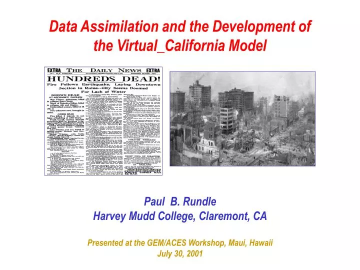
Data Assimilation and the Development of the Virtual_California Model. Paul B. Rundle Harvey Mudd College, Claremont, CA Presented at the GEM/ACES Workshop, Maui, Hawaii July 30, 2001. References.

E N D
Data Assimilation and the Development of the Virtual_California Model Paul B. Rundle Harvey Mudd College, Claremont, CA Presented at the GEM/ACES Workshop, Maui, Hawaii July 30, 2001
References P. B. Rundle, J.B. Rundle, K.F. Tiampo, J. Sa Martins, S. McGinnis and W. Klein, Nonlinear network dynamics on earthquake fault systems, Phys. Rev. Lett., in press (2001). J.B. Rundle, P. B. Rundle, W. Klein, J. Sa Martins, K.F. Tiampo, A. Donnellan and L.H. Kellogg, GEM plate boundary simulations for the plate boundary observatory: Understanding the physics of earthquakes on complex fault systems, PAGEOPH, in press (2001). P. B. Rundle, J.B. Rundle, J. Sa Martins, K.F. Tiampo, S. McGinnis, W. Klein, Triggering dynamics on earthquake fault systems, pp. 305-317, Proc. 3rd Conf. Tect. Problems San Andreas Fault System, Stanford University (2000). P. B. Rundle, J.B. Rundle, J. Sa Martins, K.F. Tiampo, S. McGinnis, W. Klein, Network dynamics of Earthquake Fault Systems, Trans. Am. Geophys. Un. EOS, 81 (48) Fall Meeting Suppl. (2000)
3D View Topology of Virtual_California 1999
3D View Topology of Virtual_California 2000
Earthquakes Used to Set Friction Values Only events larger than M > 5.8 were used.
Epicenters of historic earthquakes in Southern California since 1812 Static Data Assimilation, Step 1: Assign Seismic Moments of Earthquakes to Faults Seismic moments of paleo, historic, and instrumentally recorded large events are assigned to all faults in the model by a probability density function. jth earthquake ith fault rij-3 , the distance between the jth earthquake and the ith fault segment, is the rate at which stress amplitude falls off with distance from a dislocation. It is used as a probability density function that localizes the moment release on nearby faults.
Definition of Seismic Moment Slip-area for compact crack Difference between static & kinetic friction coefficients Static Data Assimilation, Step 2: Determination of Static-Kinetic Friction Coefficients Definitions: Mo(tj) -- Seismic moment of jth earthquake mi -- Average seismic moment resolved onto ith fault -- Shear modulus s -- Average Slip -- Static stress drop A -- Area of fault f - Fault shape factor (order ~ 1) - Average normal stress (assume gravity) s - Static friction coefficient k - Kinetic friction coefficient Assume: f ~ 1; ~ 5 x 10⁶ Pa; ~ 3 x 10¹⁰ Pa
Static Data Assimilation, Step 2: Computed Static-Kinetic Friction Coefficients At right is the result of the calculation of S - K for the Virtual_California 1999 model. This difference in friction coefficients determines the nominal values of slip on the various fault segments.
Static Data Assimilation, Step 2: Computed Static-Kinetic Friction Coefficients Above is S - K for the Virtual_California 2000 model.
F Baseline values for parameters are determined for each fault segment. It can easily be shown that: 2 = So is an observable quantity. Deng and Sykes (1997) tabulate the average fraction of stable interseismic, aseismic slip for many faults in California. > 0 Stress R Time F = 0 Stress, R Data from T Tullis, PNAS, 1996 Average stable aseismic slip Total slip Static Data Assimilation, Step 3: Aseismic Slip Factor determines fraction of total slip that is stable aseismic slip.