Download
1 / 18
260 likes | 662 Views
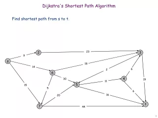
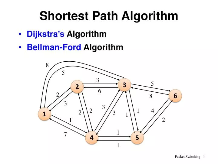
Shortest Path Algorithm. Dijkstra’s Algorithm Bellman-Ford Algorithm. 8. 5. 3. 3. 5. 2. 6. 6. 2. 8. 3. 3. 2. 1. 4. 1. 2. 3. 1. 2. 1. 1. 7. 4. 5. 1. Reduced graph. 5. 3. 3. 5. 2. 6. 2. 1. 1. 2. 3. 2. 1. 4. 5. 1. Dijkstra’s Algorithm. 2. 3. 2. 3.

E N D
Shortest Path Algorithm • Dijkstra’s Algorithm • Bellman-Ford Algorithm 8 5 3 3 5 2 6 6 2 8 3 3 2 1 4 1 2 3 1 2 1 1 7 4 5 1
Reduced graph 5 3 3 5 2 6 2 1 1 2 3 2 1 4 5 1
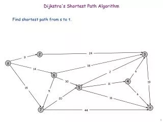
Dijkstra’s Algorithm 2 3 2 3 D2 = 2 D3 = 4 D2 = 2 D3 = 5 1 1 6 6 4 5 4 5 D4 = 1 D4 = 1 D5 = 2 T = { 1, 4 } T = { 1 } D3 = 3 2 3 2 3 D2 = 2 D3 = 4 D2 = 2 1 1 6 6 D6 = 4 4 5 4 5 D4 = 1 D5 = 2 D4 = 1 D5 = 2 T = { 1, 2, 4 } T = { 1, 2, 4, 5 }
Dijkstra’s Algorithm (cont) Node D T 2 3 4 5 6 ¥ ¥ 1 2 5 1 1, 4 ¥ 2 4 1 2 ¥ 1, 4, 2 2 4 1 2 1, 4, 2, 5 2 3 1 2 4 1, 4, 2, 5, 3 2 3 1 2 4 1, 4, 2, 5, 3, 6 2 3 1 2 4
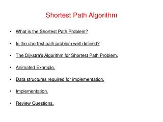
Dijkstra’s Algorithm (cont) • w(i, j) = link cost, L(n) = path cost from node s to n • 1. [Initialization] • T = {s} • L(n) = w(s, n) for n ≠ s • 2. [Get next node] • Find x Ï T such that L(x) = min L(j) • Add x to T • 3. [Update Least-Cost Paths] • L(n) = min [ L(n), L(x) + w(x, n) ] for all n Ï T • Go to step 2 jÏT
Bellman-Ford Algorithm D(2)3 = 4 2 3 2 3 D(1)2 = 2 D(1)3 = 5 D(2)2 = 2 1 1 6 6 D(2)6 = 10 4 5 4 5 D(1)4 = 1 D(2)4 = 1 D(2)5 = 2 h = 1 h = 2 D(3)3 = 3 2 3 D(3)2 = 2 1 6 D(3)6 = 4 4 5 D(3)4 = 1 D(3)5 = 2 h = 3
Bellman-Ford Algorithm (cont) Node D h 2 3 4 5 6 ¥ ¥ ¥ ¥ ¥ 0 Source = 1 ¥ ¥ 1 2 5 1 2 2 4 1 2 10 3 2 3 1 2 4 4 2 3 1 2 4
link j s n <= h links Bellman-Ford Algorithm (cont) • Lh(n) = path cost from s to n w/ no more than h links • 1. [Initialization] • L0(n) = ∞, for all n ≠ s • Lh(s) = 0, for all h • 2. [Update] • For each successive h ≥ 0 • For each n ≠ s, compute • Lh+1(n) = min [ Lh(j) + w(j, n) ] j
Comparisons L(n) = min [ L(n), L(x) + w (x, n) ] Lh(x, D) x … …… S D S D x x Dijkstra’s (Link State) Bellman-Ford (Distance Vector)
Routing in ARPANET • First generation(RIP), 1969 • Adaptive Routing is adopted • Use Bellman-Ford algorithm Distance Vector • Estimated link delay is simply the queue length for that link • Every 128ms, each node exchanges its delay vector (routing table) with all its neighbors • Information about a change in network condition would gradually ripple through the network
j k i Routing in ARPANET (cont) • Each node i maintains • di j = current estimate of min delay from i to j • si j = next node in the current min-delay route from i to j • Node k updates its vectors as follows • dk j= Min [ lk i + di j ]iÎA • sk j= i using i that minimizes the expression abovewhereA = set of neighbor nodes for klk i = current estimate of delay from k to i
Routing in ARPANET (cont) • Major shortcomings of RIP • It did not consider line speed, merely queue length. Higher capacity links were not given the favored status • Queue length is an artificial measure of delay • The algorithm was not very accurate. It responded slowly to congestion and delay increases.
Routing in ARPANET (cont) • Second generation, 1979 • Using Dijkstra’s algorithm • Link State Routing Protocol • OSPF: Open Shortest Path First protocol • The delay is measured directly • Every 10 seconds, the node computes the average delay on each outgoing link • Information of changes in delay is sent to all others nodes using flooding
Routing in ARPANET (cont) • Third generation, 1987 • Problem • The correlation between the reported values (delay) and those actually experienced after rerouting • Conclusion • Under heavy load, the goal of routing should be to give the average route a good path instead of attempting to give all routes the best path • Solution • Also consider the average utilization of links • Revisedcost function: • delay-based metric under light loads • capacity-based metric under heavy loads
Calculate Link Costs • Measure the avg. delay over the last 10 sec • Using the single-server queuing model (M/G/1), the measured delay is transformed into an estimate of link utilization • Average the link utilizationr (n+1) with the previous estimate of utilization U(n) • U(n+1) = 0.5 * r (n+1) + 0.5 * U(n) • The link cost is set as a function of average utilization
0.0 0.1 0.2 0.3 0.4 0.5 0.6 0.7 0.8 0.9 1.0 ARPANET Delay Metrics (3rd) Theoreticalqueueing delay 5 4 Delay (hops) 3 Metric for satellite link 2 Metric forterrestrial link 1 0 Estimated utilization
ARPANET Delay Metrics (3rd) • Delay is normalized to the value achieved on an idle line • The cost value is kept at the minimum value until a given level of utilization is reached • Reducing routing overhead at low traffic levels • Above a certain level of utilization, the cost level is allowed to rise to a maximum value that is equal to three times the minimum value • To dictate that traffic should not be routed around a heavily utilized line by more than two additional hops