Layout studies Tools and results – general overview

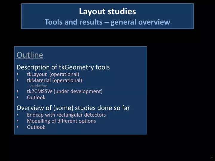
1. Outline Description of tkGeometry tools • tkLayout (operational) • tkMaterial (operational) • - validation • tk2CMSSW (under development) • Outlook Overview of (some) studies done so far • Endcap with rectangular detectors • Modelling of different options • Outlook Layout studiesTools and results – general overview

2. tkGeometry tools • tkLayout: generation of detector geometry • Starting from (relatively) small n of input parameters and assumptions • Basic geometrical validation (n of hits) • Calculation of overall basic parameters (surface, channels, power…) • tkMaterial: modelling of detector material • Simplified modelling with small n of input parameters • Creation of (additional) inactive volumes • Produce radpidity profile of radiation and interaction lengths • tkCMSSW: Creation of geometry files for CMSSW • Should be readable by IGUANA • Tracking is another story…

3. tkLayout Two configuration files • Geometry.cfg • Defines the geometry of active surfaces • Module_type.cfg • Defines which type of module populates each surface (layer/ring/disk) Some (non exhaustive) examples in the following slides

4. Definition of Tracker Volumes Tracker aRandomName { // ... } Barrel ABARREL { // ... } Generic structure of the geometry configuration file

5. Definition of Tracker Volumes Tracker aRandomName { // ... } Barrel ABARREL { // ... } Endcap SOMEDISKS { // ... } Generic structure of the geometry configuration file

6. Definition of Tracker Volumes Tracker aRandomName { // ... } Barrel ABARREL { // ... } Endcap SOMEDISKS { // ... } Barrel ANOTHERBARREL { // ... } Generic structure of the geometry configuration file

7. tkLayout Main TK parameters Tracker 2pt_ecsq { zError = 70; // spread in IP z position, mm overlap = 1; // required overlap as seen from IP, mm smallDelta = 2;// radial distance consecutive sensors along z (rphi) bigDelta = 12; // radial distance consecutive sensors along rphi (z) etaCut = 2.55; // remove detectors above cut ptCost = 200; // CHF / cm^2 stripCost = 40; // CHF / cm^2 ptPower = 0.1; // mW / channel stripPower = 0.5; // mW / channel } z rf

8. tkLayout Modules • Sensors optimally cut out of 6” wafers • Usable radius to be specified • Square sensors default • aspectRatio • Parameter to generate rectangular sensors • Option to generate smaller sensors not yet implemented

9. tkLayout Barrel geometry Space in r-z defined by • nModules • innerRadius • outerRadius N of layers • nLayers Multiplicity in f • phiSegments Radii of layers • Automatically approximated to equidistant • Can be manually adjusted through several options Overall length • Layers re-adjusted to same length, within each barrel

10. tkLayout Barrel special options Double-Stack layers • Inner stack is a shrunk clone of the outer stack • Option stacked 3/-40; • Creates a clone of layer 3, 40 mm inside Mezzanine barrels • Specify starting z position • minimumZ = 2110; N.B. Module arrangement always without Lorentz angle compensation • Feature to be added, if needed

11. tkLayout EndCap geometry Space in r • innerRadiusorinnerEta • outerRadius N of disks • nDisks Z of first and last disk given by • minimumZorbarrelGap • maximumZ Multiplicity in f • phiSegmentsas in barrel Z of intermediate disks • Automatically placed following geometrical progression • zi/zi-1 = zi+1/zi

12. tkLayout Procedure to define rings Wedge-shaped modules (default) • Shape automatically optimized (ring-by-ring) to maximize silicon sensor surface • Can be retuned (manually) in some rings, to match overall radial range Rectangular modules • Shape=rectangular; // default wedge • aspectRatio=1.1; // default 1.0 • No optimization possible • Aspect ratio tuned “by hand” • possibly for both barrel and end-caps • Overlap calculated at the tip of the module

13. tkLayout Definition of module types • For each volume, define module types as follows: BarrelType Barrel{ nStripsAcross[1] = 768; // 768 strips along rf, ≈ 110÷120 mmpitch nSides[1] = 1; // SS module (one sensor) nSegments[1] = 4; // 4-fold z segmentation (≈ 2.5 cm strip length) type[1] = rphi; // rphi, stereo, pt - name used in summaries … } • In the EndCaps, modules can be specified by rings nStripsAcross[nring] = xxx; • Or by ring and disk nStripsAcross[nring,ndisk] = xxx;

14. tkLayout One non-trivial output: occupancy estimate • Occupancy parametrized from present Tracker • From full simulation • Separately for Barrel and EndCap • Observed values reproduced to batter than 10% • Re-scaled according to channel length • Accurate for pitch ≈ 100 μm • Pessimistic (overestimated) for significantly smaller pitch • Used to evaluate needed strip length • Assuming a target occupancy within a few % • Also used to evaluate needed bandwidth • Too pessimistic: to be improved N.B. All numbers shown in the following correspond to 400 mb/BX!!

15. tkLayout Conclusions and outlook • Tool easy and fast to use • Avoids clumsy powerpoint/excel exercises • (… and/or relying too much on intuition) • Output can be easily extended to include other quantities • Multiplicities of services, electronics components etc… once input defined • Code modular, can be evolved as needed • Add new options if requested, e.g. • Module arrangement with Lorentz angle compensation • Parametrization of “cluster occupancy”, instead of channel occupancy • User-defined module size • …

16. tkMaterial • Creation of volumes • Starting from a geometry generated with tkLayout • Modelling of materials • Strategy chosen to limit complexity and maximize flexibility • Configuration file • Some examples

17. tkMaterial Volumes • Volumes are created around the active surfaces • Will receive materials related to • Modules • Services (power, cooling, readout..) • Support structures • Other volumes dedicated to services • Created automatically after analysis of tkLayout geometry • Cfr “up” and “down” configurations below • Additional volumes for support structures • Some automatic, some user-defined • … up up down

18. tkMaterial Volumes: Barrel modules P = position of the module; n = n of channels For each module type: • M=A× n(p-1) + B × n + C × (p-1) + D • D: constant amount • Examples: sensors, cooling pipes, module frame… • C: scaled with module position • Example: HV wires (accumulate from z=0 towards higher z) • B: scaled with n of channels • Example: hybrids in readout modules and their cooling contacts • A: scaled with n of channels and module position • Example: LV wires, twp for signals…. • Flag assigned to each contribution • “L” = Local; “E” = exiting • Contribution with “E” flag are taken as input for module services

19. tkMaterial Modules: examples // Sensor – does not scale M Si 0 0 0 0.2 mm L ; // Hybrid – scales with n of channels M G10 0 2.26 g 0 0 L ; M Cu 0 0.83 g 0 0 L ; // All services below calculated over 100 mm length = 1 module // 4 TWP/hybrid – scales with n of channels and module position M Cu_twp 0.132 g 0 0 0 E ; M PE_twp 0.08 g 0 0 0 E ; “M” indicates a Module volume

20. tkMaterial Volumes: EndCap modules Same concept as for barrel, but • Different rings in a disk may have different module flavours • While modules are all identical along a Barrel rod/string • Services from inner rings decrease in density while running outwards on a disk • Simple scaling with ring # does not work Solution • Explicit calculation of material from inner rings • Taking into account module types and density scaling

21. tkMaterial Volumes: Service Volumes • Service volumes receive material: • from module volumes • With user-defined scaling laws from module materials with “E” flags • from neighbour service volumes • Materials with “E” flag: everything that goes in goes out • With appropriate geometrical scaling • Done automatically by the software

22. tkMaterial Service Volumes: Examples //Manifolds D 0.79 g Steel 4.2 g Steel L; D 0.18 g CO2 1.4 g CO2 L; //Radial pipes D 0.79 g Steel 17.2 g/m Steel E; D 0.18 g CO2 3.7 g/m CO2 E; //Service holding mechanics D 0.79 g Steel 7.4 g Al L; • “D” indicates the service volume • Only “E”xiting materials from the module volumes are taken into account • Materials flagged with “E” are then propagated across service volumes

23. tkMaterial Volumes for mechanical supports • Some created automatically • e.g. inner support tube for barrel and endcap • Some user defined • e.g. support disks in Outer Barrel • N.B.All studies focused only on material inside the Tracking Volume (so far) Modules Services Support

24. tkMaterial TOB only Inside TK volume CMSSW 0 1 Validation with TOB • Spike at z=0: correct • Tiny overlap in z=0, seen or not depending on binning • Modelling of IC Bus imperfect - by choice • Causing local increase for <0.4, decrease for 0.4<<0.8 • Not necessarily so relevant for modelling next TK • Electronics at the end of the rod (CCUM, opticalconnectors, wiring…) moved just outside • Makes rising edge of the peak sharper tkMaterial

25. tkMaterial TOB only Inside TK volume CMSSW 0 1 Validation with TOB • Spike at z=0: correct • Tiny overlap in z=0, seen or not depending on binning • Modelling of IC Bus imperfect - by choice • Causing local increase for <0.4, decrease for 0.4<<0.8 • Not necessarily so relevant for modelling next TK • Electronics at the end of the rod (CCUM, opticalconnectors, wiring…) moved just outside • Makes rising edge of the peak sharper

26. tkMaterial Conclusions and outlook • Accuracy and flexibility fully adequate for present needs • Cannot model heavy objects localized in some regions of the sensor volumes (hopefully not needed!) • Very accurate (≈ %) otherwise • Could in fact be accurate enough for many years • Can be used to follow the evolution of the material estimate during the Tracker design • Can help to compare different options • And therefore help and support detector engineering • Only material inside the Tracking volume has been studied so far • There may be still problems to fix in the volumes at the TK boundaries

27. Next steps • tkLayout • Implement additional features, as needed • Notably “small” modules • tkCMSSW • Translation of geometry to xml files for CMSSW ongoing • Barrels already visibile in IGUANA; EndCaps will take longer • Discussing about validation steps • In parallel investigating reconstruction/tracking code (N. Giraud) • tkMaterial • Debug and validate volumes on boundaries • Low priority; can be relevant if translation to CMSSW is successful • All packages • Write documentation and user instructions • One brave “external” user so far, perhaps some more soon

28. Modelling of Outer Layers (readout only) Work in progress • Integration studies @CERN • Thermal modelling @ UCSB 3D design by Antonio Conde Garcia • Susanne Kyre, Dean White • First results very encouraging

29. General concepts(details given in previous presentations) • Strip length reduced to ≈ 5 or 2.5 cm to cope with particle density • Hybrids mounted on sensors. One hybrid serving two rows of strips • Pitch adapter integrated on hybrid (or on sensor) • Power through wires, data through twps, no large PCBs • Optical links (GBT) integrated at the end of the rods (periphery of disks) • GBTs receive twps from modules • Assume TOB twps, for the time being • Power converters integrated on small separate PCBs, one per hybrid • Mechanics and cooling contacts adapted from present TOB • Assume CO2 cooling • For material modelling take wires, connectors and all other elements from TOB • A priori pessimistic • Should ensure that nothing relevant is forgotten

30. Some studies on outer part • Layout taken as reference: • Outer Part: • 4 single-sided layers in the radial range 50-110 cm (barrel) • A 12-module long Barrel requires a 5 disks forward to complete rapidity coverage • In the example above: • Same rectangular modules in Barrel and End-Cap • Two versions used: 110 μm × 2.5 cm and 110 μm × 5 cm • Show results about this option, then make one step back and compare with other options 30

31. Statistics • Assumptions for power • Readout: 0.5 mW / channel • 2 W / GBT optical channel

32. Material inside tracking volume

33. One step back: EndCap with wedges • This was the starting point • Comparison of optimization procedures • EndCap with wedges • Build barrel with square modules (optimal use of of silicon), with a chosen number of modules along z • Position disks after barrel, optimize overall use of silicon in all rings (e.g. in the specific case “stretch” the shape compared to individual optimization) • EndCap with same modules as barrel • Modify aspect ratio to cover radial range with integer number of rings • Recalculate barrel • Iterate to account for second order effects • Barrel modules are not square anymore • EndCap modules have excess of overlap because of non-optimal shape • Expect penalty in n of modules, n of channels, power, material

34. Comparisons: coverage rectangles wedges Slightly better due to longer barrel

35. Wedges: statistics

36. Wedges: material

37. Comparison: numbers • Penalty in n of modules, power,material≈ 5% • Comes also with some positive features • Slightly longer barrel / slightly better coverage • Smaller pitch in barrel • Seems to be a good option!

38. Another study: barrel-only geometry for outer part • First step: build two geometries with similar coverage • The barrel-only geometry can use square detectors

39. Barrel only: statistics

40. Barrel only: material

41. Comparison: numbers • Despite the use of square sensors, the Barrel-only has a large penalty • Particularly bad at low radii • Barrel + Endcap is clearly preferable

42. Another small study: location of GBTs • GBTs at the end of the barrel • (option shown before)

43. Another small study: location of GBTs • GBTs outside the Tracking volume • (e.g. over the EndCap or on bulkhead) • Basically no change • With present assumptions material of twps ≈ material of GBTs + power wires • To be re-evaluated in future

44. Next step: modelling of PT layers • Understanding of integration aspects much more limited than for readout layers • Dedicated discussion in TUPO last week • Expect more progress in the coming weeks/months • Used as baseline the two geometries presented in the R&D proposal from Geoff/Anders • Surface similar, module material similar, power estimates compatible, data rate the same (given by functionality) • No need to distinguish between the two at this stage • Part list should be reasonably OK • Although it is not yet understood how they may come together • Some provision of material for cooling (and mechanics) • Basic assumptions recalled in the following slides

45. PT module with horizontal link sensor assembler data out control in ROC PCB ~2mm 26mm concentrator PCB f R 80mm custom part or integrated into PCB f z R-f section

46. PT module with vertical link 6*(7.2 + .8) mm • “Vertical” data transmission through substrate • Correlation logic implemented at pixel level • Dimension limited by substrate technology z 3*16 mm + 10 mm f TFEA TFEA TFEA Sensor 250 μm 150 μm 100 μm 800 μm 100 μm 150 μm 250 μm … R Substrate … other service functions 7.2 mm low profile wire bonds z Sensor R 16 mm Read Out f

47. PT module with vertical link – a variant • Same as before with different interconnection technology • Double bump assembly with through vias in the chip TFEA Sensor 250 μm C4 100 μm ASIC 100 μm C4 100 μm Substrate 700 μm C4 100 μm ASIC 100 μm C4 100 μm Sensor 250 μm … Substrate … 8.0 mm Through Via AUX ROA 16 mm

48. Part list and assumptions • Module • 2×200 μm sensor thickness • 800 μm substrate with ≈70 μm Cu • GBTs • One link / module for trigger • One link / 12 modules for readout (4 twps / module) • Power converters • 3 converters / (module + trigger GBT) • 2 converters / readout GBT • Cooling • 2 straight pipes per row of modules • Provision of some TPG and Alu for cooling contacts • Mechanics • Some CF… • Wires, connectors etc… • As in readout layers

49. Two PT layers • Layers still modelled with ≈ 10×10 cm2 sensors • Multiplicities given earlier rescaled accordingly • Along rϕ, module multiplicity in ratio 2:3 in the two layers • Convenient to define sectors

50. Statistics • N.B. PT module count in the table corresponds to ≈ 10×10 cm2 sensors • Assumptions for power • Readout: 0.5 mW / channel • PT: 0.1 mW / channel • 2 W / GBT