Download
1 / 66
660 likes | 672 Views
This article provides an in-depth analysis of texture classification and synthesis techniques, including local and global texture description methods, filter selection, scale selection, and feature extraction. It also discusses the applications and challenges of texture analysis in various fields.

E N D
Texture Some slides: courtesy of David Jacobs
Examples Simple textures (material classification): Brodatz dataset More general textures on unstructured scenes Dynamic textures
Applications • Classification (Objects and Scene, Material) • Segmentation: group regions with same texture • Shape from texture: estimate surface orientation or shape from texture • Synthesis ( Graphics) : generate new texture patch given some examples
Issues: 1) Discrimination/Analysis (Freeman)
Texture for Scene classification TextonBoost (Shotton et al. 2009 IJCV)
Texture provides shape information Gradient in the spacing of the barrels (Gibson 1957)
Texture gradient associated to converging lines (Gibson1957)
Shape from texture • Classic formulation: Given a single image of a textured surface, estimate the shape of the observed surface from the distortion of the texture created by the imaging process • Approaches estimate plane parameters, Require restrictive assumptions on the texture • isotropy (same distribution in every direction) and orthographic projection • Homogeneity (every texture window is same)
slant tilt
Texture description for recognition Two main issues • 1. Local description: extracting image structure with filters (blobs, edges, Gabors, or keypoint descriptors) ; different scales • 2. Global description: - statistical models (histograms or higher order statistics, MRF ) - Some models (networks, ant systems, etc.)
Why computing texture? • Indicative of material property -> attribute description of objects • Good descriptor for scene elements • For boundary classification: need to distinguish between object boundary and texture edges
Overview • Local: Filter selection and scale selection for local descriptors • Global: Statistical description: histogram • MFS (multifractal spectrum): invariant to geometric and illumination changes • Edge classification using texture and applying it shadow detection
Local descriptors: motivation Ideally we think of texture as consisting of texture elements (Textons) Since in real images there are no canonical elements, we apply filter that pick up “blobs” and “bars”
What are Right Filters? • Multi-scale is good, since we don’t know right scale a priori. • Easiest to compare with naïve Bayes: Filter image one: (F1, F2, …) Filter image two: (G1, G2, …) S means image one and two have same texture. Approximate: P(F1,G1,F2,G2, …| S) By P(F1,G1|S)*P(F2,G2|S)*…
What are Right Filters? • The more independent the better. • In an image, output of one filter should be independent of others. • Because our comparison assumes independence. • Wavelets seem to be best.
Blob detector • A filter at multiple scales. • The biggest response should be when the filter has the same location and scale as the blob.
Center Surround filter • When does this have biggest response? • When inside is dark •And outside is light • Similar filters are in humans and animals + - +
Blob filter • Laplacian of Gaussian: Circularly symmetric operator for blob detection in 2D Need to scale-normalize:
Efficient implementation • Approximating the Laplacian with a difference of Gaussians: (Laplacian) (Difference of Gaussians)
At fine scale At coarser scale
Filter banks • We apply a collection of multiple filters: a filter bank • The responses to the filters are collected in feature vectors, which are multi-dimensional. • We can think of nearness, farness in feature space
Filter banks orientations • What filters to put in the bank? • Typically we want a combination of scales and orientations, different types of patterns. “Edges” “Bars” scales “Spots” Leung Malik filterbank: 48 filters: 2 Gaussian derivative filters at 6 orientations and 3 scales, 8 Laplacian of Gaussian filters and 4 Gaussian filters. Matlab code available for these examples: http://www.robots.ox.ac.uk/~vgg/research/texclass/filters.html
Gabor Filters Gabor filters at different scales and spatial frequencies top row shows anti-symmetric (or odd) filters, bottom row the symmetric (or even) filters.
Gabor filters are examples of Wavelets • We know two bases for images: • Pixels are localized in space. • Fourier are localized in frequency. • Wavelets are a little of both. • Good for measuring frequency locally.
Global: descriptions • Simplest histograms
Global description: Simplest Texture Discrimination • Compare histograms. • Divide intensities into discrete ranges. • Count how many pixels in each range. 0-25 26-50 51-75 76-100 225-250
High-dimensional features • Often a texture dictionary is learned first by clustering the feature vectors using K-mean clustering. • Histogram, where each cluster is represented by cluster center, called textons • Each pixel is assigned to closest texton • Histograms are compared (often with Chi-square distance)
… 2. Learning the visual vocabulary Slide credit: Josef Sivic
… 2. Learning the visual vocabulary Clustering Slide credit: Josef Sivic
Example of texton dictionary Filterbank (13 filters) Universal textons (64) Image Texton map (color-coded) Martin, Fowlkes, Malik, 2004: Berkeley (Pb) edge detector
Texture recognition histogram Universal texton dictionary Julesz, 1981; Cula & Dana, 2001; Leung & Malik 2001; Mori, Belongie & Malik, 2001; Schmid 2001; Varma & Zisserman, 2002, 2003; Lazebnik, Schmid & Ponce, 2003
Chi square distance between texton histograms Chi-square i 0.1 j k 0.8 (Malik)
Different approaches • Universal texton dictionaries vs Different dictionaries for each texture class • Sparse features vs. dense features • Different histogram comparisons e.g L1 distance or EMD (earth mover’s distance)
Multi-fractal spectrum (MFS) texture signature A framework to combine local and global description based on multi-fractal-spectrum theory • Invariant to surface and view-point changes • Robust to Illumination changes • Compact vector size (~70 vs~1000) • Computational efficient • Simplicity in the implementation Y. Xu, H. Ji and C. Fermüller, Viewpoint invariant texture description using fractal Analysis, International Journal of Computer Vision, 2009 Y. Xu,et al , " Scale-space texture description on SIFT-like textons," Computer Vision and Image Understanging, 2012
Fractal dimension • Measurement at scale δ. For each δ we measure an object in a way that ignores regularity of size less than δ, and we see how these measurement behaves as δ goes to 0. • Most natural phenomena satisfy the power law: an estimated quantity is proportional to with D a constant (for example the length of a coastline) for a point set E in R2 Fractal dimension
Fractal dimension D = 1 D = 2 D = 1.7
MFS • Extension: divide quantity into a discrete number of sets, compute fd for every set -> MFS. e.g. divide intensity [1, 255] into 26 classes.
Invariance • The MFS is invariant under the bi-Lipschitz transform; basically any smooth function-> translation, rotation, projective transformation, warpings of the surfaces • Illumination variance Consider the intensity function I(x) piecewise locally linear : akI(x) + bk MFS defined on edges is invariant
Basic idea • Multiple MFSs from multiple density functions defined on different local feature spaces. • Local feature spaces • Zero-mean intensity • Gradient energy • Laplacian energy Spatial distortion invariance Illumination invariance
View-point invariance Grass Bulrush Trees
(cont’) Trees Brush Grass MFS on feature space