A Survey of Various Propagation Models for Mobile Communication

1. A Survey of Various Propagation Models for Mobile Communication Tapan K Sarkar, Zhong Ji, Kyungjung Kim, Abdellatif Medouri, and Magdalena Salazar-Palma IEEE Antenna and Propagation Magazine, Vol. 45, No. 3, June 2003 Presented by Lu-chuan Kung (kung@uiuc.edu)

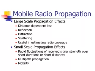
2. Outline • Mobile radio propagation • Models for Path Loss • Empirical (statistical) models • Site-specific (deterministic) models • Models for Small-scale Fading • Impulse-Response Models

3. Mobile Radio Propagation • EM wave • Radio Wave Propagation: • Reflection • Diffraction • Scattering • Multi-path channel impulse response

4. Basic Definitions • Path Loss • Friis free-space equation • Metrics (dBm, mW) • P(dBm) = 10 * log[ P(mW) ] • Power-Delay Profile • Take spatial average of |hb(t;τ)|2 over a local area

5. Basic Definitions • Time-Delay Spread • First-arrival delay (τA) • Mean excess delay • RMS delay

6. Inter-symbol Interference • Slide from R. Struzak

7. Basic Definitions • Coherence Bandwidth • Range of frequency over which channel is “flat” • Relation to delay spread • Doppler spread • Measure spectral broadening caused by motion of the mobile • Coherence Time • Time duration over which channel impulse response is invariant

8. Models of Path Loss • Log-distance Path Loss Model • Log-normal Shadowing • Xσ: N(0,σ) Gaussian distributed rv

9. Models for Path LossEmpirical Models • Okumura Model • L50: median of propagation path loss • LF: free-space propagation loss • Amu(f,d): median attenuation • G(hte), G(hre): gain factors for BS and mobile antenna • GAREA: environment gain • Applicable frequncies: 150 MHz to 1920 MHz (typically is extrapolated up to 3000 MHz) • Disadvantage: slow response to rapid changes in terrain

10. Models for Path LossEmpirical Models • Dual-slope model • P1=PL(d0): the path loss at d0 • dbrk: Fresnel breakpoint • Lb: basic transmission-loss parameter • n1,n2: slopes of the best-fit line before and after dbrk

11. Models for Path LossEmpirical Models: Indoor Case • Indoor Log-distance path loss model • FAF(q): floor attenuation factor • WAF(p): wall attenuation factor

12. Models for Path LossEmpirical Models: Indoor Case • Indoor Log-distance path loss model • γ ranges from 1.5 to 4 • γ depends on frequency and building materials

13. Site-specific Path Loss ModelsRay-tracing • Ray-tracing Technique • Assume energy is radiated through infinitesimally small tubes, often called rays • Model signal propagation via ray propagation

14. Ray-tracing Technique:Image Method • Image Method • Images of a source serve as secondary sources • N reflecting planes • N first-order images • N(N-1) two-reflection images • N(N-1)(N-1) three-reflection images • Efficient but cannot handle complex environments

15. Ray-tracing Technique:Brute-force Method • Brute-force Method • Considers a bundle of transmitted rays • Generates reflecting and refracting rays when hits an object • Generates a family of diffracting rays when hits a wedge

16. Ray-tracing Model • 2-D Ray-tracing model • Each ray is a ray sector of sector angle φ • Smallerφprovides higher accuracy • 3-D model • Each ray tube occupy the same solid angle • Antenna patterns are incorporated

17. Site-specific Path Loss Model:FDTD Models • Ray-tracing fails for complex lossy structures with finite dimentions • Finite-Difference Time-Domain (FDTD) method • Solve Maxwell’s equations numerically • Complete solution for all points in the map • Requires large computational resources

18. Site-specific Path Loss Model: Artificial Neural-Network Models • Artificial Neural-Network Models (ANNs) • Use neural network models to predict path loss from noisy measurements • Pros: • Better accuracy than statistical model • Better computational efficiency than other site-specific models • Cons: • Slow convergence • Unpredictable solutions during learning

19. Models for Small-Scale Fading • Rayleigh fading • Assume a large number of scattering sources • By Central Limit Theorem, signal is a Gaussian rv with random phase between 0~2π • The power (envelope) of this random Gaussian vector is Rayleigh distributed

20. An Example of Rayleigh Fading • A typical Rayleigh fading envelope at 900MHz, mobile unit velocity = 120km/hr

21. Models for Small-Scale Fading • Ricean Distribution • A: peak amplitude of the dominant signal • I0(): modified Bessel function of the first kind • Add a dominant LOS signal to Rayleigh fading • Ricean factor: K=A2/2σ2

22. Models for Small-Scale Fading • Log-normal Fading • m: median value • σ: standard deviation

23. Models for Small-Scale Fading • Suzuki Model • Combines log-normal and Rayleight distributions

24. Models for Small-Scale Fading • Nakagami Model • r: envelope amplitutde • Ω=<r2>: time-averaged power of received signal • m: the inverse of normalized variance of r2 • Get Rayleigh when m=1

25. Impulse-Response Models • Complete characterization of the linear system • Model the effect of multi-path fading • Measurement-based Models • Statistical Models • Deterministic Models

26. Impulse-Response Models Measurement-based Models: • Minimum resolvable delay = probing pulse width Tbb • Subject to interference and noise Direct Pulse Measurement

27. Impulse-Response Models: Measurement-based Models • Spread-spectrum Sliding Correlator

28. Impulse-Response Models: Measurement-based Models • Swept-frequency measurements • Pros: • Provide both amplitude and phase information • Cons: • Require hardwired synchronization between TX and RX • Need fast sweeping times but reduces time resolution

29. Impulse-Response Models:Statistical Models • Two-ray Rayleigh Fading Model • α1 & α2: independent Rayleigh r.v. • θ1 & θ2 ~ Uni[0, 2π] • τ: time delay between the two rays

30. Impulse-Response Models:Statistical Models • SIRCIM Model • Based on measurements at 1300MHz in 5 factory and other buildings • Model power-delay profile as a piecewise function For LOS: For OBS:

31. Conclusion • With propagation models, we can • Provide installation guidelines • Mitigate interference • Design better wireless system