Download
1 / 15
150 likes | 290 Views
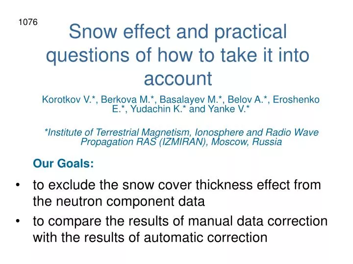
1076. Snow effect and practical questions of how to take it into account. Korotkov V.*, Berkova M.*, Basalayev M.*, Belov A.*, Eroshenko E.*, Yudachin K.* and Yanke V.* *Institute of Terrestrial Magnetism, Ionosphere and Radio Wave Propagation RAS (IZMIRAN), Moscow, Russia. Our Goals:

E N D
1076 Snow effect and practical questions of how to take it into account Korotkov V.*, Berkova M.*, Basalayev M.*, Belov A.*, Eroshenko E.*, Yudachin K.*and Yanke V.* *Institute of Terrestrial Magnetism, Ionosphere and Radio Wave Propagation RAS (IZMIRAN), Moscow, Russia Our Goals: • to exclude thesnow cover thickness effect from the neutron component data • to compare the results of manual data correction with the results of automatic correction
Count rates of the based station S and thestation with snow N (1) where
The basic detector choice MCRL IGY NM64 Jungfraujoch
The method of the snow effect exclusion Basing on (1) variations relative to the base period corrected on the snow effect and expressed by way of the measured variations can be entered as: (2) For thedefinition of the variations corrected on the snow effectby themeasured variations it is necessary to estimate theefficiency. For that we’ll get the data of the detectorregistering nearly the same variations as the detectorwith snow. If thiscondition apply to some average time interval it ispossible to write: or (3)
Data averaging and filtration Approximation by polynomialshas been done for a polynomial of enough high degree m, where n - a number of hour in a month. A moving average prime filterin spite of its simplicityis optimal for the majority of tasks. The moving averagefilter equation is put down as where - the constant weight factor or in the recursive form after the first step of calculations
The Gaussian high-cut filter TheGaussian high-cut filter is a moving average filter inwhich the Gaussian function is applied as a weightfunction. It is realized as The weight factors are preset as and the normalizing factor as The value of the distribution dispersion defines therequired width of the distribution.
Count rate variations of the based station S (Moscow)and MCRL for the March 2009 Automatic data correction – blue curve manual data correction - dottedcurve
Magadan station Distorted by the snow effect and corrected data during November 2008 – April 2009. Black curve for Gaussian smoothing, grey curve – polynominal smoothing. The based station – Moscow. We can estimate the effective snow cover thicknessas The efficiency (top curve) and the snow cover thickness (bottom). November 2008 – April 2009.
ESOI station Distorted by the snow effect and corrected dataof ESOI station during August 2007 - July 2008. Thebased station is Rome. Efficiency (top curve) and the snow cover thickness(bottom curve) for the ESOI station during August2007 - July 2008.
ESOI station On the top - the automatic (black curve) and themanual (red curve) corrections for March 2009 for theESOI station. On the bottom - the uncorrected data withsnow effect.
Jungfraujoch station Jungfraujoch IGY NM64
Jungfraujoch station Distorted by the snow effect and corrected data of the Jungfraujoch station (3nm64) during January - December 2008. The based stations are Jungfraujoch - 18IGY (black curve) and Rome (grey curve). Efficiency (top curve) and the snow cover thickness (bottom curve) for the Jungfraujoch station (3nm64) during January 2008 - December 2008.
Conclusions • The method of exclusion of the snow cover thickness effect from the data basing on the comparison of the variations of tested and based stations was tested for some stations: Magadan, ESOI and Jungfraujoch. • For this purpose the high-cut filters has been applied. While selecting the filter degree the compromise choice between spasmodic signal change and its sufficient slow change with several days period had to be done. By default the effective width of the filter is about 24 hours. • The snow effect can be excluded from the data with the accuracy is about 0.3-0.4%. The ideal case is when the detectors are identical and are in the same point. • The described method allows not only to exclude the snow effect but also to make an estimate of the effective snow cover thickness. • The method can be applied in real time too ifuse one-sided filters. • We did not find out any advantages of the Gaussian filter over the moving average filter.