Download
1 / 10
100 likes | 200 Views
Sorting “Example” with Insertion Sort. i = 5 A E M P X L E. i = 1 E X A M P L E. i = 2 E X A M P L E. i = 6 A E L M P X E. i = 3 A E X M P L E. i = 7 A E E L M P X. i = 4 A E M X P L E. Closest Pair Pseudo-code. ClosestPair(P[1..n])

E N D
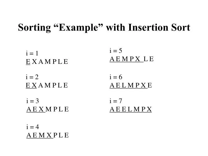
Sorting “Example” with Insertion Sort i = 5 A E M P X L E i = 1 E X A M P L E i = 2 E X A M P L E i = 6 A E L M P X E i = 3 A E X M P L E i = 7 A E E L M P X i = 4 A E M X P L E
Closest Pair Pseudo-code ClosestPair(P[1..n]) //input: P[1..n] a collection of points sorted by the x coordinates //output: Points r and s, with r≠ s, such that distance(r,s) is the shortest distance among all pairs of points in P If (n == 2) then return (P[1],P[2]) C1 Select(P[1..mid],c,d) C2 Select(P[mid+1..n],c,d) for each k in C1 do Cand candidates(k,C2,d) //at most 6 points will be in D for each ca in Cand do if distance(k,ca) < d) then d distance(k,ca) (r,s) (k,ca) return (r,s) mid floor(n/2) c (P[mid].x + P[mid+1].x)/2 (a,b) ClosestPair(P[1..mid]) (w,z) ClosestPair(P[mid+1..n]) d1 distance(a,b) d2 distance(w,z) if (d1 < d2) then (r,s,d) (a,b,d1) else (r,s,d) (w,z,d2)
size in bits of a pointer Graph Representations G = (E,V) D E A F C B G H Adjacency lists vs. Adjacency Matrix (Pages 29, 30) |V|2 |V| + k × 2 × |E| Size
Depth-First Search • Initially all nodes are marked with 0 (non visited). • Every node that is visited will be marked with a value of 1 or more • The number marking a node indicates its depth relative to other marked nodes • Complexity: Adjacency Lists: O(|V| + |E|) Adjacency Matrix: O(|V|2)
Breadth-First Search • Initially all nodes are marked with 0 (non visited). • Every node that is visited will be marked with a value of 1 or more • Use a queue (FIFO policy) to control order of visits • Complexity: Adjacency Lists: O(|V| + |E|) Adjacency Matrix: O(|V|2)
Questions about Graphs • Is the graph connected? • Find the connected components of the graph • Is the graph acyclic? • Find articulation points • Find minimum-number of edges
Applications of Graphs • In many problems, the graphs are not constructed apriori because they would be extremely large. • In such situations while the system is solving a problem, it is constructing the graph as-needed. • Example of such a problem: Computer-generated Game plan
Planning: Simple Example A B C C A B Initial Goal (on A Table) (on C A) (on B Table) (clear B) (clear C) (on C Table) (on B C) (on A B) (clear A)
Search Space: A Graph! C A B C A B C B A B A C B A C B A B C C B A B A C A C A A B C B C C B A A B C
Homework (Optional) • 5.2: 2, 1.b, 4, 6, 7, 10