Download
1 / 40
400 likes | 582 Views
High dynamic range imaging. Camera pipeline. 12 bits. 8 bits. Short exposure. 10 -6. 10 6. dynamic range. Real world radiance. 10 -6. 10 6. Picture intensity. Pixel value 0 to 255. Long exposure. 10 -6. 10 6. dynamic range. Real world radiance. 10 -6. 10 6. Picture

E N D
Camera pipeline 12 bits 8 bits
Short exposure 10-6 106 dynamic range Real world radiance 10-6 106 Picture intensity Pixel value 0 to 255
Long exposure 10-6 106 dynamic range Real world radiance 10-6 106 Picture intensity Pixel value 0 to 255
Recovering High Dynamic Range Radiance Maps from Photographs Paul E. DebevecJitendra Malik SIGGRAPH 1997
Recovering response curve 12 bits 8 bits
• 2 • 2 • 2 • 2 • 2 • 3 • 3 • 3 • 3 • 3 • 1 • 1 • 1 • 1 • 1 Recovering response curve Image series Dt =2 sec Dt =1 sec Dt =1/2 sec Dt =1/4 sec Dt =1/8 sec 255 0
Idea behind the math Each line for a scene point. The offset is essentially determined by the unknown Ei
Idea behind the math Note that there is a shift that we can’t recover
Recovering response curve • The solution can be only up to a scale, add a constraint • Add a hat weighting function
Constructing HDR radiance map combine pixels to reduce noise and obtain a more reliable estimation
Gradient Domain High Dynamic Range Compression RaananFattalDaniLischinski Michael Werman SIGGRAPH 2002
log derivative attenuate integrate exp The method in 1D
The method in 2D • Given: a log-luminance image H(x,y) • Compute an attenuation map • Compute an attenuated gradient field G: • Problem: Gmay not be integrable!
Poisson equation Solution • Look for image I with gradient closest to G in the least squares sense. • I minimizes the integral:
Attenuation log(Luminance) gradient magnitude attenuation map
interpolate X = interpolate X = Multiscale gradient attenuation
Informal comparison Bilateral[Durand et al.] Photographic[Reinhard et al.] Gradient domain[Fattal et al.]
Informal comparison Bilateral[Durand et al.] Photographic[Reinhard et al.] Gradient domain[Fattal et al.]
Informal comparison Bilateral[Durand et al.] Photographic[Reinhard et al.] Gradient domain[Fattal et al.]
Local Laplacian Filters :Edge-aware Image Processingwith a Laplacian Pyramid Sylvain Paris Samuel W. Hasinoff Jan Kautz SIGGRAPH 2011
Background on Gaussian Pyramids • Resolution halved at each level using Gaussian kernel level 3 (residual) level 2 level 1 level 0
Background on Laplacian Pyramids • Difference between adjacent Gaussian levels level 3 (residual) level 2 level 1 level 0
Intuition for 1D Edge • Decomposition for the sake of analysis only • We do not compute it in practice = + + Input signal Discontinuity Texture Smooth
Intuition for 1D Edge = + + Input signal Discontinuity Texture Smooth Does notcontribute toLap. pyramid at that scale(d2/dx2=0)
Ideal Texture Increase Discontinuity Texture Keep unchanged Amplify
Our Texture Increase σ σ σ σ Input signal Local nonlinearity “Locally good”version user-defined parameter σdefines texture vs. edges
Our Texture Increase = + + “Locally good” Only left sideis affected Discontinuity Unaffected Texture Left side is ok, right side is not Smooth Does notcontribute toLap. pyramid at that scale(d2/dx2=0)
Negligible becausecollocated with discontinuity Negligible becauseGaussian kernel ≈ 0 Discussion = + + “Locally good” Only left sideis affected Discontinuity Unaffected Texture Left side is ok, right side is not Smooth Does notcontribute toLap. pyramid at that scale(d2/dx2=0) Good approximation to ideal case overall (formal treatment in paper)