A Fully Polynomial Time Approximation Scheme for Timing Driven Minimum Cost Buffer Insertion

1. A Fully Polynomial Time Approximation Scheme for Timing Driven Minimum Cost Buffer Insertion Professor Shiyan Hu, Ph.D. Department of Electrical and Computer Engineering Michigan Technological University

2. Moore’s law Twice the number of transistors, approximately every two years 2

3. Interconnect Delay Dominates Gate Delay 3

4. Technology Scaling 130nm 65nm • Global interconnect lengths does not shrink • Local interconnect lengths shrink • Delay ∝ RC • Resistance R =rL/S, where S is reduced • Capacitance C slightly changes 4

5. Interconnect Delay Scaling • Scaling factor s=0.7 per generation • Emore Delay of a wire of length l tint= (rl)(cl)/2= rcl2/2 (first order) • Local interconnects tint : (r/s2)(c)(ls)2/2 = rcl2/2 • Local interconnect delay is roughly unchanged • Global interconnects tint : (r/s2)(c)(l)2/2= rcl2 • Global interconnect delay doubles which is unsustainable • Interconnect delay increasingly more dominant 5

6. Timing Driven Buffer Insertion 6

7. Buffers Reduce RC Wire Delay x x/2 x/2 x/2 R C rx/2 R rx/2 cx/4 cx/4 cx/4 cx/4 C ∆t ∆t = t_buf – t_unbuf = RC + tb– rcx2/4 x 7

8. Intuitive Analysis L Interconnect Elmore delay = rcL2/2 l=2 l l l (Of course, we need to consider buffer delay) 8

9. L r,c – Resistance, cap. per unit length Rd – On resistance of inverter Cg – Gate input capacitance l Detailed Analysis • The delay of a wire of length L is T=rcL2/2 • Assume N identical buffers with equal inter-buffer length l(L = Nl). To minimize delay 9

10. Quadratic Delay -> Linear Delay • Substituting lopt back into the interconnect delay expression: Delay grows linearly with L instead of quadratically. This is why buffer insertion is highly effective and thus widely used for reducing circuit delay. 10

11. 25% Gates are Buffers Saxena, et al. [TCAD 2004] 11

12. ITRS Projections 12

13. Problem Formulation • Steiner Tree • n candidate buffer locations T Minimal cost (area/power) solution 13

14. Solution Characterization • To model effect to downstream, a candidate solution is associated with • v: a node • C: downstream capacitance • Q: required arrival time • W: cumulative buffer cost 14

15. Candidate Buffering Solutions 15

16. Candidate solutions are propagated toward the source Dynamic Programming (DP) • Start from sinks • Candidate solutions are generated • Three operations • Add Wire • Insert Buffer • Merge • Solution Pruning 16

17. Solution Propagation: Add Wire x (v1, c1, w1, q1) (v2, c2, w2, q2) • c2 = c1 + cx • q2 = q1 - (rcx2/2 + rxc1) • r: wire resistance per unit length • c: wire capacitance per unit length 17

18. Solution Propagation: Insert Buffer (v1, c1, w1, q1) (v1, c1b, w1b, q1b) • q1b = q1 - d(b) • c1b = C(b) • w1b = w1 + w(b) • d(b): buffer delay 18

19. Solution Propagation: Merge (v, cl , wl , ql) (v, cr, wr, qr) • cmerge= cl + cr • wmerge= wl+ wr • qmerge = min(ql, qr) 19

20. Example of Solution Propagation (v, C, Q, W) • r = 1, c = 1 • Rb = 1, Cb = 1, tb = 1 • Rd = 1 2 2 (v1, 1, 20, 0) Add wire (v2, 3, 16, 0) (v2, 1, 12, 1) v1 v1 Insert buffer Add wire Add wire (v3, 5, 8, 0) (v3, 3, 8, 1) v1 v1 slack = 3 slack = 5 Add driver Add driver 20

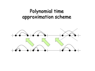
21. Solution Propagation (1) (2) (3) 21

22. Exponential Runtime 2 solutions 4 solutions 8 solutions 16 solutions n candidate buffer locations lead to 2n solutions 22

23. Too Many Solutions • Needs solution pruning for acceleration • Two candidate solutions • (v, c1, q1,w1) • (v, c2, q2,w2) • Solution 1 is inferior to Solution 2 if • c1 c2 : larger load • and q1 q2 : tighter timing • and w1w2: larger cost 23

24. Car Race - Speed END Car Speed <=> RAT 24

25. Car Race - Load Load <=> Load Capacitance 25

26. Faster & Smaller Load Faster & smaller load (larger RAT, smaller capacitance): Good END Slower & larger load (smaller RAT, larger capacitance): Inferior 26

27. Faster & Larger Load: Result 1 END 27

28. Faster & Larger Load: Result 2 END Who will be the winner? Cannot tell at this moment, so keep both of them. 28

29. inferior/dominated if C1 C2,W1 W2 and Q1 Q2 Pruning (Q1,C1,W1) • Non-dominated solutions are maintained: for the same Q and W, pick min C • # of solutions depends on # of distinct W and Q, but not their values (Q2,C2,W2) 29

30. Generating Candidates (1) (2) (3) 30

31. Pruning Candidates (3) (b) (a) Both (a) and (b) look the same to the source. Remove the one with the worse slack and cost (4) 31

32. Candidate Example Continued (4) (5) 32

33. Candidate Example Continued After pruning (5) At driver, compute the candidate solution satisfying the timing target with minimum cost. The result is optimal. 33

34. Branch Merge Left Candidates Right Candidates 34

35. Pruning During Branch Merge (n1n2) solutions after each branch merge. Worst-case ((n/m)m) solutions. With pruning 35

36. Gap Selected Milestone Works on Timing Buffering Is it possible to design a provably good algorithm running in polynomial time with theoretical guarantee on the error to the optimal solution? NP-hardness proof Lillis’ algorithm Shi and Li’s algorithm van Ginneken’s algorithm 1990 1991 ……. 1996 ……. 2003 2004 ……. 2008 2009 This is a major open problem for a decade! 36

37. Bridging The Gap A Fully Polynomial Time Approximation Scheme (FPTAS) • Provably good • Computes a solution with cost at most (1+ɛ) of the optimal cost for any ɛ>0 • Runs in time polynomial in n (nodes), b (buffer types) and 1/ɛ • Best solution for an NP-hard problem in theory • Highly practical We are bridging the gap! 37

38. The Rough Picture W*: the cost of optimal solution Make guess on W* Not Good Check it Good (close to W*) Return the solution Key 1: Efficient checking Key 2: Smart guess 38

39. Key 1: Efficient Checking Benefit of guess • Only maintain the solutions with cost no greater than the guessed cost • This is the first reason for acceleratation 39

40. The Oracle • Oracle (x): the checker, able to decide whether x>W* or not • Without knowing W* • Answer efficiently 40

41. Construction of Oracle(x) Scale and round each buffer cost Dynamic Programming Only interested in whether there is a solution with cost up to x satisfying timing constraint Perform DP to scaled problem with cost upper bound n/ɛ. Time polynomial in n/ɛ 41

42. Scaling and Rounding Buffer cost xɛ/n 2xɛ/n 3xɛ/n 4xɛ/n 0 42

43. Scaling and Rounding • Rounding error at each buffer xɛ/n, total rounding error xɛ. • Larger xɛ/n: larger error, fewer distinct costs and faster • Smaller xɛ/n: smaller error, more distinct costs and slower • Rounding is the second reason for acceleration # distinct buffer costs is at most O(n/ε) since only solutions with W bounded by n/ɛ are propagated. Buffer cost 2 3 0 1 4 43

44. Oracle Construction Run dynamic programming with cost  n/ɛ • Yes, there is a solution satisfying timing constraint • No, no such solution • With cost rounded and scaled back, the solution has cost at most n/ɛ • xɛ/n + xɛ= (1+ɛ)x > W* • With cost rounded and scaled back, the solution has cost at least n/ɛ •xɛ/n = x  W* 44

45. Rounding on Q • # solutions bounded by # distinct W and Q • # W = O(n/ɛ1), ɛ1 is used for W • Rounding before DP • # Q • Round up Q to nearest value in {0, ɛ2T/m , 2ɛ2T/m, 3ɛ2T/m,…,T }, in branch merge (m is # sinks) • Rounding during DP • # Q = O(m/ɛ2), ɛ2 is used for Q • Rounding error bounded by ɛ2T/m per branch merge, by ɛ2T for the whole tree • # non-dominated solutions is O(mn/ɛ1ɛ2) 0 ɛ2T/m 2ɛ2T/m 3ɛ2T/m 4ɛ2T/m 45

46. Q-W Rounding Before Branch Merge Q T 4ɛ2T/m 3ɛ2T/m 2ɛ2T/m ɛ2T/m W 0 1 2 3 4 n/ɛ1 46

47. Buffer Insertion Runtime 47

48. Branch Merge Runtime - 1 When merging Wl=2 with Wr=1, previously we need to try quadratic # of combinations, now only linear # of combinations. Target Q=0 48

49. Branch Merge Runtime - 2 Target Q= ɛ2T/m 49

50. Branch Merge Runtime - 3 Target Q= 2ɛ2T/m 50