Download
1 / 47
480 likes | 677 Views
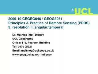
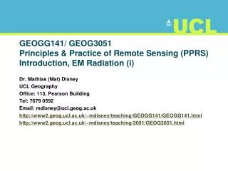
GEOGG141 Principles & Practice of Remote Sensing (PPRS) RADAR III: Applications Revision. Dr. Mathias (Mat) Disney UCL Geography Office: 113, Pearson Building Tel: 7670 0592 Email: mdisney@ucl.geog.ac.uk www.geog.ucl.ac.uk /~ mdisney. RECAP. Observations of forests.

E N D
GEOGG141Principles & Practice of Remote Sensing (PPRS) RADAR III: ApplicationsRevision Dr. Mathias (Mat) Disney UCL Geography Office: 113, Pearson Building Tel: 7670 0592 Email: mdisney@ucl.geog.ac.uk www.geog.ucl.ac.uk/~mdisney
Observations of forests... • C-band (cm-tens of cm) • low penetration depth, leaves / needles / twigs • L-band • leaves / branches • P-band • can propagate through canopy to branches, trunk and ground • C-band quickly saturates (even at relatively low biomass, it only sees canopy); P-band maintains sensitivity to higher biomass as it “sees” trunks, branches, etc • Low biomass behaviour dictated by ground properties
Surfaces - scattering depends on moisture and roughness • Note - we could get penetration into soils at longer wavelengths or with dry soils (sand) • Surfaces are typically • bright if wet and rough • dark if dry and smooth • What happens if a dry rough surface becomes wet ? • Note similar arguments apply to snow or ice surfaces. • Note also, always need to remember that when vegetation is present, it can act as the dominant scatterer OR as an attenuator (of the ground scattering)
EasternSahara desert Landsat SIR-A Penetration 1 – 4 m
Safsaf oasis, Egypt Penetration up to 2 m Landsat SIR-C L-band 16 April 1994
Single channel data • Many applications are based on the operationally-available spaceborne SARs, all of which are single channel (ERS, Radarsat, JERS) • As these are spaceborne datasets, we often encounter multi-temporal applications (which is fortunate as these are only single-channel instruments !) • When thinking about applications, think carefully about “where” the information is:- • scattering physics • spatial information (texture, …) • temporal changes
Multi-temporal data • Temporal changes in the physical properties of regions in the image offer another degree of freedom for distinguishing them but only if these changes can actually be seen by the radar • for example - ERS-1 and ERS-2:- • wetlands, floods, snow cover, crops • implications for mission design ? • ALOS-PALSAR (2005-2011) revisits
Wetlands in Vietnam - ERS Oct 97 Jan 99 18 Mar 99 27 May 99 Sept 99 Dec 99 Jan 00 Feb 00
SIR-C (mission 1 left, mission 2 centre, difference in blue on right)
Floods... Maastricht A two date composite of ERS SAR images 30/1/95 (red/green) 21/9/95 (blue)
Snow cover... Glen Tilt - Blair Atholl ERS-2 composite red = 25/11/96 cyan=19/5/97 Scott Polar Research Institute
Agriculture Gt. Driffield Composite of 3 ERS SAR images from different dates
OSR - Oil seed rape WW - Winter wheat
ERS SAR East Anglia
Radar modelling • Surface roughness • Volume roughness • Dielectric constant ~ moisture • Models of the vegetation volume, e.g. water cloud model of Attema and Ulaby, RT2 model of Saich Multitemporal SHAC radar image Barton Bendish
Water cloud model A – vegetation canopy backscatter at full cover B – canopy attenuation coefficient C – dry soil backscatter D – sensitivity to soil moisture σ0 = scattering coefficient ms = soil moisture θ = incidence angle L = leaf area index Vegetation
Simulated backscatter r2 = 0.81
Canopy moisture r2 = 0.96
Applications • Irrigation fraud detection • Irrigation scheduling • Crop status mapping, e.g. disease, water stress
Multi-parameter radar • More sophisticated instruments have multi-frequency, multi-polarisation radars, with steerable beams (different incidence angle) • Also, different modes • combinations of resolutions and swath widths • SIR-C / X-SAR • ENVISAT ASAR, ALOS PALSAR,...
Flevoland April 1994 (SIR-C/X-SAR) (L/C/X composite) L-total power (red) C-total power (green) X-VV (blue)
Thetford, UK AIRSAR (1991) C-HH
Thetford, UK AIRSAR (1991) multi-freq composite
Coherent RADAR modelling Thetford, UK SHAC (SAR and Hyperspectral Airborne Campaign) http://badc.nerc.ac.uk/view/neodc.nerc.ac.uk__ATOM__dataent_11742960559518010 Disney et al. (2006) – combine detailed structural models with optical AND RADAR models to simulate signal in both domains http://www.sciencedirect.com/science/article/pii/S0034425705003445 Drat optical model + CASM (Coherent Additive Scattering Model) of Saich et al. (2001)
Coherent RADAR modelling Thetford, UK SHAC (SAR and Hyperspectral Airborne Campaign) http://badc.nerc.ac.uk/view/neodc.nerc.ac.uk__ATOM__dataent_11742960559518010 Disney et al. (2006) – combine detailed structural models with optical AND RADAR models to simulate signal in both domains http://www.sciencedirect.com/science/article/pii/S0034425705003445 Drat optical model + CASM (Coherent Additive Scattering Model) of Saich et al. (2001)
Optical signal with age for different tree density (HyMAP optical data)
OPTICAL RADAR
An ambitious list of Applications... • Flood mapping, Snow mapping, Oil Slicks • Sea ice type, Crop classification, • Forest biomass / timber estimation, tree height • Soil moisture mapping, soil roughness mapping / monitoring • Pipeline integrity • Wave strength for oil platforms • Crop yield, crop stress • Flood prediction • Landslide prediction
CONCLUSIONS • Radar is very reliable because of cloud penetration and day/night availability • Major advances in interferometric SAR • Should radar be used separately or as an adjunct to optical Earth observation data? ALOS (RIP)
Revision • Exam: 3 hrs, answer 4 from 7 (2 from Dietmar, 5 from me) • Types of question based on PREVIOUS material be similar each year (not surprisingly!) • Planck function, orbital calculations, definitions of terms, pre-processing stages • Factors controlling measured signal from vegetation across vis/SWIR, or angular behaviour • RADAR principles eg RADAR equation, resolutions • Principles of SAR interferometry and applications • General questions - systems to address a given problem • KEY: address that problem • Does Q give scope for moving beyond one platform or wavelength? If so then DO SO…
Revision • Types of question based on NEW material for 2011 • LiDAR • Principles of lidar remote sensing? • What is it good for and limitations? • Example applications • Radiative Transfer modelling • Basis of RT model – building blocks? • Structure, leaf scattering, soil scattering • Scalar RT equation • what do terms mean? • How can we go about solving?
Radiant energy from 0 to Total radiant energy for =0 to = Revision problems: Planck’s Law • Fractional energy from 0 to F0? Integrate Planck function • Note Eb(,T), emissive power of bbody at , is function of product T only, so....
3 l m l T ( mK x10 ) F ( T) ® l 0 (dimensionless) 2 .067 3 .273 4 .481 5 .634 6 .738 8 .856 10 .914 12 .945 14 .963 16 .974 18 .981 20 .986 Revision: Planck’s Law example • Q: what fraction of the total power radiated by a black body at 5770 K fall, in the UV (0 0.38µm)? • Need table of integral values of F0 • So, T = 0.38m * 5770K = 2193mK • Or 2.193x10³mK i.e. between 2 and 3 • Interpolate between F0(2x10³) and F0(3x10³) • Finally, F00.38 = 0.193*(0.273-0.067)+0.067 = 0.11 • i.e. ~11% of total solar energy lies in UV between 0 and 0.38m
Orbits: examples • Orbital period for a given instrument and height? • Gravitational force Fg = GMEms/RsE2 • where G is universal gravitational constant (6.67x10⁻¹¹ Nm2kg2); ME is Earth mass (5.983x1024kg); ms is satellite mass (?) and RsE is distance from Earth centre to satellite i.e. 6.38x10⁶ + h where h is satellite altitude • Centripetal (not centrifugal!) force Fc = msvs2/RsE • where vs is linear speed of satellite (=sRsE where is the satellite angular velocity, rad s-1) • for stable (constant radius) orbit Fc = Fg • GMEms/RsE2 = msvs2/RsE = ms s2RsE2 /RsE • so s2 = GME /RsE3 From:http://csep10.phys.utk.edu/astr161/lect/history/kepler.html
Orbits: examples • Orbital period T of satellite (in s) = 2/ • (remember 2 = one full rotation, 360°, in radians) • and RsE = RE + h where RE = 6.38x10⁶ m • So now T = 2[(RE+h)3/GME]1/2 • Example: geostationary altitude? T = ?? • Rearranging: h = [(GME /42)T2 ]1/3 - RE • So h = [(6.67x10-11*5.983x1024/42)(24*60*60)2 ]1/3 - 6.38x10⁶ • h = 42.2x10⁶ - 6.38x106 = 35.8km
Orbits: examples • Example: polar orbiter period, if h = 705x103m • T = 2[(6.38x10⁶ +705x103)3 / (6.67x10-11*5.983x1024)]1/2 • T = 5930.6s = 98.8mins • Example: show separation of successive ground tracks ~3000km • Earth angular rotation = 2/24*60*60 = 7.27x10⁻⁵rads s-1 • So in 98.8 mins, point on surface moves 98.8*60*7.27x10-5 = .431 rads • Remember l =r* for arc of circle radius r & in radians • So l = (Earth radius + sat. altitude)* • = (6.38x10⁶ +705x103)* 0.431 = 3054km