Download
1 / 27
270 likes | 471 Views
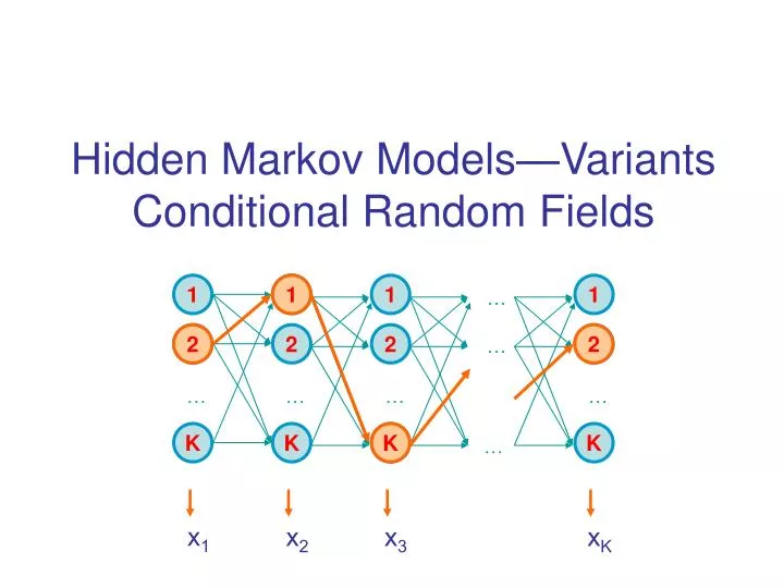
1. 2. 2. 1. 1. 1. 1. …. 2. 2. 2. 2. …. K. …. …. …. …. x 1. K. K. K. K. x 2. x 3. x K. …. Hidden Markov Models—Variants Conditional Random Fields. Two learning scenarios. Estimation when the “right answer” is known Examples:

E N D
1 2 2 1 1 1 1 … 2 2 2 2 … K … … … … x1 K K K K x2 x3 xK … Hidden Markov Models—VariantsConditional Random Fields
Two learning scenarios • Estimation when the “right answer” is known Examples: GIVEN: a genomic region x = x1…x1,000,000 where we have good (experimental) annotations of the CpG islands GIVEN: the casino player allows us to observe him one evening, as he changes dice and produces 10,000 rolls • Estimation when the “right answer” is unknown Examples: GIVEN: the porcupine genome; we don’t know how frequent are the CpG islands there, neither do we know their composition GIVEN: 10,000 rolls of the casino player, but we don’t see when he changes dice QUESTION: Update the parameters of the model to maximize P(x|)
1. When the “true” parse is known Given x = x1…xN for which the true = 1…N is known, Simply count up # of times each transition & emission is taken! Define: Akl = # times kl transition occurs in Ek(b) = # times state k in emits b in x We can show that the maximum likelihood parameters (maximize P(x|)) are: Akl Ek(b) akl = ––––– ek(b) = ––––––– i AkicEk(c)
2. When the “true parse” is unknown Baum-Welch Algorithm Compute expected # of times each transition & is taken! Initialization: Pick the best-guess for model parameters (or arbitrary) Iteration: • Forward • Backward • Calculate Akl, Ek(b), given CURRENT • Calculate new model parameters NEW : akl, ek(b) • Calculate new log-likelihood P(x | NEW) GUARANTEED TO BE HIGHER BY EXPECTATION-MAXIMIZATION Until P(x | ) does not change much
Higher-order HMMs • How do we model “memory” larger than one time point? • P(i+1 = l | i = k) akl • P(i+1 = l | i = k, i -1 = j) ajkl • … • A second order HMM with K states is equivalent to a first order HMM with K2 states aHHT state HH state HT aHT(prev = H) aHT(prev = T) aHTH state H state T aHTT aTHH aTHT state TH state TT aTH(prev = H) aTH(prev = T) aTTH
Modeling the Duration of States 1-p Length distribution of region X: E[lX] = 1/(1-p) • Geometric distribution, with mean 1/(1-p) This is a significant disadvantage of HMMs Several solutions exist for modeling different length distributions X Y p q 1-q
Solution 1: Chain several states p 1-p X Y X X q 1-q Disadvantage: Still very inflexible lX = C + geometric with mean 1/(1-p)
Solution 2: Negative binomial distribution Duration in X: m turns, where • During first m – 1 turns, exactly n – 1 arrows to next state are followed • During mth turn, an arrow to next state is followed m – 1 m – 1 P(lX = m) = n – 1 (1 – p)n-1+1p(m-1)-(n-1) = n – 1 (1 – p)npm-n p p p 1 – p 1 – p 1 – p Y X(n) X(1) X(2) ……
Example: genes in prokaryotes • EasyGene: Prokaryotic gene-finder Larsen TS, Krogh A • Negative binomial with n = 3
Solution 3: Duration modeling Upon entering a state: • Choose duration d, according to probability distribution • Generate d letters according to emission probs • Take a transition to next state according to transition probs Disadvantage: Increase in complexity of Viterbi: Time: O(D) Space: O(1) where D = maximum duration of state F d<Df xi…xi+d-1 Pf Warning, Rabiner’s tutorial claims O(D2) & O(D) increases
Viterbi with duration modeling emissions emissions Recall original iteration: Vl(i) = maxk Vk(i – 1) akl el(xi) New iteration: Vl(i) = maxk maxd=1…DlVk(i – d) Pl(d) akl j=i-d+1…iel(xj) F L d<Df d<Dl Pl Pf transitions xi…xi + d – 1 xj…xj + d – 1 Precompute cumulative values
Conditional Random Fields A brief description of a relatively new kind of graphical model
1 1 1 1 … 2 2 2 2 … … … … … K K K K … Let’s look at an HMM again 1 Why are HMMs convenient to use? • Because we can do dynamic programming with them! • “Best” state sequence for 1…i interacts with “best” sequence for i+1…N using K2 arrows Vl(i+1) = el(i+1) maxk Vk(i) akl = maxk( Vk(i) + [ e(l, i+1) + a(k, l) ] ) (where e(.,.) and a(.,.) are logs) • Total likelihood of all state sequences for 1…i+1 can be calculated from total likelihood for 1…i by only summing up K2 arrows 2 2 K x1 x2 x3 xN
1 1 1 1 … 2 2 2 2 … … … … … K K K K … Let’s look at an HMM again 1 • Some shortcomings of HMMs • Can’t model state duration • Solution: explicit duration models (Semi-Markov HMMs) • Unfortunately, state i cannot “look” at any letter other than xi! • Strong independence assumption: P(i | x1…xi-1, 1…i-1) = P(i | i-1) 2 2 K x1 x2 x3 xN
1 1 1 1 … 2 2 2 2 … … … … … K K K K … Let’s look at an HMM again 1 • Another way to put this, features used in objective function P(x, ): • akl, ek(b), where b • At position i: all K2akl features, and all K el(xi) features play a role • OK forget probabilistic interpretation for a moment • “Given that prev. state is k, current state is l, how much is current score?” • Vl(i) = Vk(i – 1) + (a(k, l) + e(l, i)) = Vk(i – 1) + g(k, l, xi) • Let’s generalize g!!! Vk(i – 1) + g(k, l, x, i) 2 2 K x1 x2 x3 xN
“Features” that depend on many pos. in x i-1 i • What do we put in g(k, l, x, i)? • The “higher” g(k, l, x, i), the more we like going from k to l at position i • Richer models using this additional power • Examples • Casino player looks at previous 100 pos’ns; if > 50 6s, he likes to go to Fair g(Loaded, Fair, x, i) += 1[xi-100, …, xi-1 has > 50 6s] wDON’T_GET_CAUGHT • Genes are close to CpG islands; for any state k, g(k, exon, x, i) += 1[xi-1000, …, xi+1000 has > 1/16 CpG] wCG_RICH_REGION x7 x8 x9 x10 x1 x2 x3 x4 x5 x6
“Features” that depend on many pos. in x x7 x8 x9 x10 x1 x2 x3 x4 x5 x6 Conditional Random Fields—Features • Define a set of features that you think are important • All features should be functions of current state, previous state, x, and position i • Example: • Old features: transition kl, emission b from state k • Plus new features: prev 100 letters have 50 6s • Number the features 1…n: f1(k, l, x, i), …, fn(k, l, x, i) • features are indicator true/false variables • Find appropriate weights w1,…, wn for when each feature is true • weights are the parameters of the model • Let’s assume for now each feature has a weight wj • Then, g(k, l, x, i) = j=1…nfj(k, l, x, i) wj
“Features” that depend on many pos. in x x7 x8 x9 x10 x1 x2 x3 x4 x5 x6 Define Vk(i): Optimal score of “parsing” x1…xi and ending in state k Then, assuming Vk(i) is optimal for every k at position i, it follows that Vl(i+1) = maxk [Vk(i) + g(k, l, x, i+1)] Why? Even though at pos’n i+1 we “look” at arbitrary positions in x, we are only “affected” by the choice of ending state k Therefore, Viterbi algorithm again finds optimal (highest scoring) parse for x1…xN
1 2 3 4 5 6 … x1 x2 x3 x4 x5 x6 1 2 3 4 5 6 … x1 x2 x3 x4 x5 x6 “Features” that depend on many pos. in x • Score of a parse depends on all of x at each position • Can still do Viterbi because state i only “looks” at prev. state i-1 and the constant sequence x HMM CRF
How many parameters are there, in general? • Arbitrarily many parameters! • For example, let fj(k, l, x, i) depend on xi-5, xi-4, …, xi+5 • Then, we would have up to K | |11 parameters! • Advantage: powerful, expressive model • Example: “if there are more than 50 6’s in the last 100 rolls, but in the surrounding 18 rolls there are at most 3 6’s, this is evidence we are in Fair state” • Interpretation: casino player is afraid to be caught, so switches to Fair when he sees too many 6’s • Example: “if there are any CG-rich regions in the vicinity (window of 2000 pos) then favor predicting lots of genes in this region” • Question: how do we train these parameters?
Conditional Training • Hidden Markov Model training: • Given training sequence x, “true” parse • Maximize P(x, ) • Disadvantage: • P(x, ) = P( | x)P(x) Quantity we care about so as to get a good parse Quantity we don’t care so much about because x is always given
Conditional Training P(x, ) = P( | x)P(x) P( | x) = P(x, ) / P(x) Recall F(j, x, ) = # times feature fj occurs in (x, ) = i=1…N fj(k, l, x, i) ; count fj in x, In HMMs, let’s denote by wj the weight of jth feature: wj = log(akl) or log(ek(b)) Then, HMM: P(x, ) =exp[j=1…n wj F(j, x, )] CRF: Score(x, ) =exp[j=1…n wj F(j, x, )]
Conditional Training In HMMs, P( | x) = P(x, ) / P(x) P(x, ) =exp[j=1…n wjF(j, x, )] P(x) = exp[j=1…n wjF(j, x, )]=: Z Then, in CRF we can do the same to normalize Score(x, ) into a prob. PCRF( | x) = exp[j=1…n wjF(j, x, )]/ Z QUESTION: Why is this a probability???
Conditional Training • We need to be given a set of sequences x and “true” parses • Calculate Z by a sum-of-paths algorithm similar to HMM • We can then easily calculate P( | x) • Calculate partial derivative of P( | x) w.r.t. each parameter wj (not covered—akin to forward/backward) • Update each parameter with gradient descent! • Continue until convergence to optimal set of weights P( | x) = exp[j=1…n wjF(j, x, )]/ Z is convex!!!
Conditional Random Fields—Summary • Ability to incorporate complicated non-local feature sets • Do away with some independence assumptions of HMMs • Parsing is still equally efficient • Conditional training • Train parameters that are best for parsing, not modeling • Need labeled examples—sequences x and “true” parses (Can train on unlabeled sequences, however it is unreasonable to train too many parameters this way) • Training is significantly slower—many iterations of forward/backward