Download
1 / 29
300 likes | 424 Views
Statistical analysis of global temperature and precipitation data. Imre Bartos, Imre Jánosi Department of Physics of Complex Systems Eötvös University. The GDCN database Correlation properties of temperature data Short-term Long-term Nonlinear Cumulants Extreme value statistics

E N D
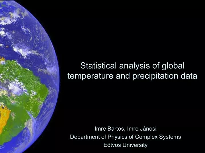
Statistical analysis of global temperature and precipitation data Imre Bartos, Imre Jánosi Department of Physics of Complex Systems Eötvös University
The GDCN database • Correlation properties of temperature data • Short-term • Long-term • Nonlinear • Cumulants • Extreme value statistics • Recent results • Degrees of Freedom estimation Outline
Temperature stations Precipitation stations 32857 stations… Global Daily Climatology Network 1950-2000
Ti Short-term correlation Long-term correlation Correlation properties
Ti Short-term correlation Long-term correlation Correlation properties Autoregressive process: ai+1 = Ti+1 - Ti+1 = F(ai) + i Linear case: AR1 ai+1 = A ai + i Short term memory: exponential decay C1() = aiai+ ~ A
Short-term correlation ai+1 = A ai + i in terms of temperature change: ai+1 = ai+1 – ai ~ Ti+1 – Ti = (A-1) ai + i thus the response function one measures: ai+1 = (A-1) ai + 0 The fitted curve: ai+1 = c1 ai + c0 Király, Jánosi, PRE (2002).
Short-term correlation ai+1 = c1 ai + c0 c1 • |c1| it increases to the South-East • c0!= 0 significantly ai - asymmetric distribution c0 Bartos, Jánosi, Geophys. Res. Lett. (2005).
Do these two effects compensate each other? Global warming (?) Short-term correlation • more warming steps (Nm) then cooling (Nh) • the average cooling steps (Sh) are bigger then the average warming steps (Sm) • Warming index: • W = (Nm Sm) / (Nh Sh) asymmetric distribution Bartos, Jánosi, Geophys. Res. Lett. (2005).
Ti Short-term correlation Long-term correlation Correlation properties Long term memory: power decay C() = aiai+ ~ -
Long-term correlation C() = aiai+ ~ - Measurement: Detrended Fluctuation Analysis (DFA) F(n) ~ n = 2 (1 - ) Asymptotic gradient () 0 ~ short term memory Initial gradient (0) ~ long-term memory DFA curve:
Detrended Fluctuation Analysis (DFA) Király, Bartos, Jánosi, Tellus A (2006). All time series are long term correlated
Nonlinear correlation Two-point correlation: C2 = aiaj, q-point correlation: Cq = F(aiajak…) Linear (Gauss) process:Cq>2 = f(C2) (3rd or higher cumulants are 0) C2 completely describes the process Nonlinear (multifractal) process: 3rd or higher cumulants are NOT 0 the 2-point correlation doesn’t give the full picture One needs to measure the nonlinear correlations for the full description
Nonlinear correlation ai |ai+1 - ai| „volatility” time series: The 2-point correlation of the volatility time series features the nonlinear correlation properties of the anomaly time series volatility - DFA exponent
Nonlinear correlation There is also short- and long-term memory for the volatility time series volatility - initial DFA exponent
In short… Daily temperature values are correlated in both short and long terms and both linearly and nonlinearly. We constructed the geographic distributions for these properties, and described or explained some of them in details. volatility - initial DFA exponent
Cumulants - nonuniform can affect the EVS skewness kurtosis
Extreme value statistics • we want to use temperature time series • temperature • anomaly • normalized anomaly
Extreme value statistics • we try to get rid of the spatial correlation lets use one station in every 4x4 grid
Explanation: preliminary filtering of „outliers” Daily normalized distribution Dangers in filtering for extreme value statistics • after filtering out the flagged (bad) data: • cutoff at 3.5 s seems exactly like a Weibull distribution
Extreme value statistics Then how can we filter out bad data?? There are certainly bad data in the series. The usual way to filter them out is to flag the suspicious ones, but it seems we cannot use the flags. One try to find real outliers: Temperature difference distribution Impossible to validate
Extreme value statistics Another possible way: try to isolate unreliable stations Also notice the two peaks Now we use all the data without filtering spatial correlations
Extreme value statistics New problem: the two peaks What makes the average maximum values differ for some stations? Why two peaks? skewness kurtosis correlation depends doesn’t depend doesn’t depend
Extreme value statistics New problem: the two peaks Average yearly maximum One can spatially separate the different peaks
Extreme value statistics Separate one peak by using US stations only: Finally we get to the Gumbel distribution
Degrees of Freedom Why does the average maximum value not depend on the correlation exponent? One can calculate the degrees of freedome of N variables with long time correlation characterized by correlation exponent g DOF = N^2 / Sli^2 Where li is the ith eigenvalue of the covariance matrix, containing the covariance of each pair of days of the year. Long term correlation: C(|x-y|) = c * |x-y|^g Short term correlation: Ti+1 = A * Ti + noise Variables determining the DOF: c, g, A.
Degrees of Freedom – Dependence on correlation C = 1 C = 0.25 Short-term C = 0.0001
Degrees of Freedom – measurement and calculation Estimation with with c=1 (underestimation) Measurement: Chi square method (underestimation)
Degrees of Freedom – difficulties It is hard to measure anything due to the bad signal to noise rato c = 1 estimation: this causes the difference To say something about c: correlation between consequtive years
Statistical analysis of global temperature and precipitation data Imre Bartos, Imre Jánosi Department of Physics of Complex Systems, Eötvös University