Download
1 / 42
430 likes | 608 Views
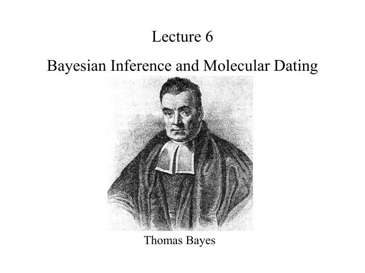
Lecture 6 Bayesian Inference and Molecular Dating. Thomas Bayes. Bayesian Inference : The explanation with the highest posterior probability. 1. Definition of conditional probability. Pr( A and B ) = Pr( A ) Pr( B A ) = Pr( B ) Pr( A B ) .

E N D
Lecture 6 Bayesian Inference and Molecular Dating Thomas Bayes
Bayesian Inference: The explanation with the highest posterior probability 1. Definition of conditional probability Pr(A and B) = Pr(A) Pr(BA) = Pr(B) Pr(AB) Prior probability, the probability of the hypothesis on previous knowledge 2. Bayes’ Theorem Likelihood function, probability of the data given the hypothesis Pr(H) Pr(DH) Pr(HD) = Pr(D) Posterior probability, the probability of the hypothesis given the data Unconditional probability of the data, a normalizing constant ensuring the posterior probabilities sum to 1.00
Odds ratios are the simplest usage for Bayes’ theorem Felsenstein’s example: He gives his prior belief in “martians” Pr(H) = 1/4. A space probe sent to mars has probability of 1/3 of finding martians if they are there. It finds none, so Pr(D H) = 1/3, where H is that martians exist is 1/3 Pr(H) Pr(DH) 1/4 1/3 = = 1/12 Pr(HD) = Pr(D) 1 Assuming all the data is correct
When the prior is a probability distribution, the posterior probability can be given as a probability distribution (often considered a density distribution under a curve) Flat prior Skewed Prior Prior 0 24 Parameter value 0 24 Parameter value
Influence of the Prior diminishes if the likelihood ratio between hypotheses increases with data collection 10 coin tosses, 3 heads 100 coin tosses, 30 heads Posterior 0 0.2 0.4 0.6 0.8 1.0 0 0.2 0.4 0.6 0.8 1.0 pheads pheads “heads” “tails”
Bayesian inference in phylogenetics First use in phylogenetics: Li (1996, PhD thesis), Rannala and Yang (1996) A useful property of Bayesian inference for phylogenetics is that with flat priors (all hypotheses equal before the data is examined), posterior probabilities for two trees are proportional to their likelihood ratio. Posterior Likelihood Prior Tree1 Tree2 Tree3 Tree1 Tree2 Tree3 Tree1 Tree2 Tree3
Bayesian inference in phylogenetic notation Prior distribution Likelihood distribution Posterior distribution (ti) (Dti) (tiD) = ti = Treei = substitution model b = branch-length (tj) (Dtj) T J=1 Where (D ti) = b(Dti,b, ) (b, ) dbd Summing over this integral becomes too complex with so many tree/parameter hypotheses
Markov chain Monte Carlo (MCMC) analysis New state rejected New state accepted Tree 1 Tree 2 The chain Tree 3 Generation: 1 2 3 4 5 6 Bayesian Posterior Probability for Tree 1 (BPPtree 1)= 4/6 Sampling the MCMC provides a valid approximation for the posterior distribution of trees (over 100,000s – 1,000,000s of generations) - without having to know the denominator
Metropolis-Hastings algorithm (the proposal mechanism) 1. Start at a random (or predetermined) tree, Ti 2. Randomly select a tree that is a neighbour in tree space, the proposal tree, Tj 3 4 1 4 1 3 e.g. 2 5 2 5 Pr(Tj) Pr(D Tj ) 3. Compute the acceptance ratio R = Pr(Ti) Pr(D Ti ) 4. If R ≥ 1, accept Tj 5. If R < 1, randomly draw from 0-1, if < R, accept Tj 6. Otherwise reject Tj and keepTi 7. Return to step 2
Useful properties of MCMC for Bayesian inference • Given an efficient proposal mechanism and sufficient generations, the MCMC with reach an equilibrium distribution • The problem of summing across all hypotheses cancels out in the acceptance ratio for Tj /Ti • The section of the MCMC that is “finding its way” towards the equilibrium distribution (the burnin) can be discarded - it is not a valid approximation for the posterior probability
Metropolis-coupled MCMC (MC3) n chains, of which n-1 are “heated” such that they can more easily move across peaks and valleys in the landscape of trees. After all n chains have gone one step a swap between randomly chosen chains is proposed (in much the same way as between generations). If accepted the two chains switch states. The cold chain (which could be stuck in a local optimum) can escape when a proposed swap with a hot chain is successful.
Sampling three simultaneous chains(MrBayes 3.0: Heulsenbeck and Ronquist, 2001) Generation chain 1 chain 2 chain 3 4100 -- (-15395.901) (-15376.724) [-15367.235] 4200 -- (-15395.854) (-15377.874) [-15368.146] 4300 -- (-15381.440) [-15376.072] (-15368.164) 4400 -- (-15375.695) (-15369.686) [-15369.127] 4500 -- [-15374.458] (-15372.051) (-15370.876) 4600 -- [-15358.899] (-15366.374) (-15365.927) 4700 -- [-15350.419] (-15366.082) (-15366.168) 4800 -- (-15369.614) [-15368.152] (-15369.902) Proposing new trees along individual chains and swapping trees between chains (to more efficiently explore tree space)
Inference is based only on sampling from the cold chain - for which the acceptance ratio for changes between generations is appropriate for approximating the posterior probability. tree tree_1 [p = 0.455, P = 0.455] (Ostrich,Rhea,(Moa,(Kiwi,(Emu,Cassowary)))) tree tree_2 [p = 0.215, P = 0.670] (Ostrich,(Kiwi,(Moa,Rhea)),(Emu,Cassowary)) tree tree_3 [p = 0.118, P = 0.788] (Ostrich,Moa,(Rhea,(Kiwi,(Emu,Cassowary))) tree tree_4 [p = 0.081, P = 0.869] (Ostrich,(Moa,Rhea),(Kiwi,(Emu,Cassowary))) tree tree_5 [p = 0.050, P = 0.919] (Ostrich,Kiwi,(Moa,(Rhea,(Emu,Cassowary)))) Rhea Ostrich Kiwi Moa From Phillips, unpub. Emu Cassowary
Squamata A Return to the Turtle example Amphibia (outgroup) H2: Diapsida H3: Archosauria H1: Anapsida Aves Mammalia Crocodilia
Bayesian inference in MrBayes 3.0 • The same data matrix as for the likelihood example (16 taxa, 3110 nucleotides) • GTR+I+ model (AIC recommendation in ModelTest) • Four MC3 chains (3 are “hot”): 2,000,000 generations • sample every 1000th tree from the “cold” chain
Discard the 1st 250,000 generations as the “burnin” +------------------------------------------------------------+ -25419.04 | *****************************************************| | ** | | | | * | | * | | * | | | | | | * | | | | | | | |* | | | | | +------+-----+-----+-----+-----+-----+-----+-----+-----+-----+ -33441.42 ^ ^ 1 10000 Estimated marginal likelihood = -25423.76 (arithmetic mean) = -25451.08 (harmonic mean) Equilibrium distribution likelihood generations 2,000,000
Model parameter summaries for the 1750 samples from the MCMC chain 95% Cred. Interval -------------------- Parameter Mean Variance Lower Upper Median -------------------------------------------------------------- TL 2.513384 0.005489 2.373000 2.663000 2.512000 r(G<->T) 1.000000 0.000000 1.000000 1.000000 1.000000 r(C<->T) 14.895438 2.952511 11.968691 18.597121 14.745678 r(C<->G) 0.088475 0.004142 0.011433 0.241428 0.074255 r(A<->T) 2.489403 0.105833 1.952249 3.220099 2.453488 r(A<->G) 8.309381 0.935429 6.684136 10.510313 8.229202 r(A<->C) 2.481878 0.108561 1.928505 3.190486 2.453910 pi(A) 0.323330 0.000044 0.310754 0.336207 0.323446 pi(C) 0.215915 0.000035 0.204413 0.227673 0.216025 pi(G) 0.209200 0.000035 0.197702 0.221016 0.209162 pi(T) 0.251555 0.000037 0.239747 0.263308 0.251377 alpha 1.017169 0.015644 0.785668 1.261082 1.013706 pinvar 0.226459 0.000787 0.164235 0.274568 0.229746 --------------------------------------------------------------
Unlike likelihood, for which parameters are optimised, Bayesian inference gives a Posterior density distribution for parameter values (integrated over all trees sampled from the chain) 95% credible interval frequency 0 0.2 0.4 Proportion of invariant sites
Statistic Mean Estimated sample size Sampling analysis (e.g. Tracer 1.0) Rambaut and Drummond All ESS should be at least >100
Has the MCMC run for sufficient generations? Have the chains converged on similar likelihood values and swaps being made between each of them? Do different runs of the same analyses converge? Sampling over generation plots reveal that likelihoods have levelled (equilibrium distribution is reached) Estimated sample sizes for all parameters are >100, indicating substantial coverage of parameter space
Bayesian inference tree with Posterior probabilities Amphibia Salamander Caecilian 1.00 Skink Iguana 1.00 Green Turtle 1.00 Painted Turtle Diapsidia Alligator 1.00 1.00 Archosauria Caiman 0.99 Cassowary 1.00 1.00 Penguin 1.00 Platypus Echidna 1.00 Mammalia 1.00 Dog 3 toed Sloth 0.79 1.00 Kangaroo Opossum
Tree 1 Tree 3 Amphibia Amphibia Turtles Mammalia Mammalia Squamates Squamates Turtles Birds Birds Crocodilia Crocodilia Tree 2 Tree1 Tree2 Tree3 -lnL +36.1 +11.7 <best> KH 0.002 0.044 -- SH 0.003 0.153 -- AU 0.001 0.054 -- NPBP 0.005 0.041 -- SOWH <0.001 <0.001 -- BPP <0.001 <0.001 -- Amphibia Mammalia Turtles Squamates Birds Crocodilia
Controversies with Bayesian inference 1. Flat prior? It depends on perspective Priors for the same branch lengths (under a Jukes-Cantor model) 0.0 0.25 0.5 0.75 0 1 2 3 4 5 Branch-length as the probability of change Branch-length as expected substitutions per site
2. A flat prior on branch-lengths is not a flat prior on clade probabilities A flat prior across all topologies for the whole tree favours the largest and smallest clades over clades of intermediate taxon inclusion However, the influence on posterior probabilities maybe quite small Pickett and Randle (MPE, 2005)
3. Bounds on priors Prior 0.0 Branch-length 100 MLE Posterior 95% credible interval 0.0 Branch-length 100 A zero to infinity “bound” provides a worst case scenario
4. Bayesian posterior probabilities tend to overestimate clade support (underestimate sampling effects) when the substitution model is misspecified – Which is essentially always when using biological datasets True Simmons et al. (MBE, 2004)
Bayesian inference methods are now being incorporated into phylogenetic analysis of morphological data (a.) (b.) vpg mc sf mc sp glenoid (gl) orientation Supraspinous fossa (sf) sp vpg mc fused to scapular vpg points venteral ap relative to gl ap ap gl if gl if a. 0 0 1 0 0 b. 0 1 1 1 1 medial medial Right scapula of an echidna (a.) and a marsupial cat(b) in distal view. ap, acromion process; gl, glenoid; if, infraspinous fossa; mc, metacoracoid; sf, supraspinous fossa; sp, scapular spine; vpg, ventral process of glenoid.
Oak ATGACCGCTGCCAG Ash ACGCTCGCCATCAG Maple ATGCTCGCTACCGG glenoid (gl) orientation Supraspinous fossa (sf) mc fused to scapular vpg points venteral ap relative to gl Transitions at six sites, only one transversion is observed An ML model would allow for different transition and transversion substitution rates a. 0 0 1 0 0 b. 0 1 1 1 1 The Assumption for Likelihood that sites evolve by common mechanisms is not clear for morphological data The state “1” for one character does not mean the same thing as state “1” for another character
Lewis (Syst. Biol., 2001) recognized that ML estimation of branch-lengths could help interpret the nature of morphological change among taxa (e.g. as resulting from shared ancestry or convergence) • Mkv model for morphology resembles Jukes-Cantor (JC): • All states assumed to have the = equilibrium frequency • Changes between all states are equally probable • Differences: • Multiple (>4) states allowed • conditional on no characters being constant across all taxa
The root of the Australidelphian marsupial tree Australasian Marsupiarnivora dasyurids bandicoots diprotodonts S. American marsupials
Syndactyla diprotodonts syndactylus bandicoots dasyurids Non-syndactylus S. American marsupials
Phillips et al. (Syst. Biol, 2006) ML, MP and Bayesian inference on 17,864 nuclear and mitochondrial nucleotide sites Australasian Marsupicarnivora
Horovitz and Sánchez-Villagra (Cladistics, 2002) Parsimony on 230 morphological characters Syndactyla + Dromiciops
Mayulestes Bayesian inference (Mkv-model) on the 230 morphological characters of Horovitz and Sánchez-Villagra (2002) Pucadelphys Shrew opossum Monito del monte Pygmy possum Sugar glider Ringtail possum Cuscus Brushtail possum Tree kangaroo Pademellon Kangaroo Forest wallaby Wombat Koala Australasian Marsupicarnivora Mulgara Quoll Phascogale Marsupial mole Spiny bandicoot Long-nosed bandicoot Virginia opossum Grey Short-tailed opossum
Combined Molecular and Morphological data analysis Taxon1 ACGTAAGTC 0000110 Taxon2 ATGGAAATT 1110302 Taxon3 ACATAAATC 1020111 Taxon4 ACGCTAGTC 0010012 Partition 1 (e.g. GTR model) Partition 2 (Mkv model) (ti) (D1ti) (D2ti) (tiD12) = (tj) (D1tj) (D2tj) T J=1 Allows model-based estimation for molecular sequences to be combined with morphological data (including for fossil taxa)
Combined (DNA/morphology) Bayesian analysis of Metazoans Deuterostomes (inc. echinoderms, sea squirts, vertebrates) Ecdysozoa (inc. arthropods, nematodes) (Platyhelminthes, rotifers, acorn worms) Lophotrochozoa (inc. molluscs, annalids) Glenner et al. (Curr. Biol., 2005)
Bayesian character state reconstruction: Shell hairs on the Trochulus snails Pfenninger et al. (BMC Evol. Biol., 2005)
Relaxed-clock Bayesian Phylogenetics r = rate (substitutions/site/time); t = node height; branch-length (b) = rt; n = number of taxa A. Clock B. No-clock C. Relaxed-clock b4 b7 t4rl b3 b3 t2rj b2 b4 b2 b1 t1ri t3rk b1 b5 b6 Forces a molecular clock (r is constant) – assumes deviation from this is sampling error. Rates are influenced by sampling error and vary according to an underlying distribution (e.g. exponential or lognormal). Different rate for each branch – no sampling error is assumed.
A. Clock B. No-clock C. Relaxed-clock b4 b7 t4rl b3 b3 t2rj b2 b4 b2 b1 t1ri t3rk b1 b5 b6 n-1 node heights and 1-2 rate distribution parameters n-1 branch-length parameters 2n-3 branch-length parameters Most sequence datasets have not evolved in a clock-like fashion, and so the assumption of a clock often produces incorrect tree topologies
Relaxed-clocks : the holy grail of phylogenetics? • By allowing for the influence of sampling error, relaxed-clock models can more accurately infer underlying substitution rates and hence provide greater phylogenetic accuracy. • By estimating fewer branch-length parameters, less variance will tend to be associated with relaxed-clock model estimates, thus providing for greater phylogenetic precision than no-clock models • However, we need to know how well fitting the rate distribution models are
Drummond et al. (PLoS Biol., 2006) A. B. C. D. E. A. Bacteria (102) B. Yeasts (106) C. Plants (61) D. Animals (99) E. Primates (500)
Relaxed phylogenetics allows co-estimation of phylogeny and divergence timing Drummond et al. (PLoS Biol., 2006)