Download
1 / 70
740 likes | 1.03k Views
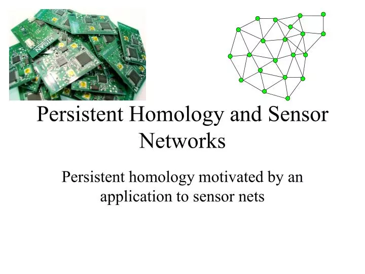
Persistent Homology and Sensor Networks. Persistent homology motivated by an application to sensor nets. Outline. A word about sensor nets Basic coverage criterion Better coverage criterion using persistence Introduce Persistent Homology Correspondence Theorem Computing the groups!

E N D
Persistent Homology and Sensor Networks Persistent homology motivated by an application to sensor nets
Outline • A word about sensor nets • Basic coverage criterion • Better coverage criterion using persistence • Introduce Persistent Homology • Correspondence Theorem • Computing the groups! • Other Applications
August 29, 2005 Hurricane Katrina hits New Orleans
Result: Useful sensor network • Measure conditions on the ground at many locations • Relay messages to and from rescue workers • Instant infrastructure • Low power/auto-power • Cheap!?
Other uses of sensor networks • Environmental monitoring • Security systems • Battlefield monitoring and communications • Large mechanical systems • Find Sarah Connor
Hole in sensor coverage area Sarah Connor escapes!
Identifying holes in the network • De Silva and Ghrist have developed a method for identifying gaps in sensor coverage • Method is based on Algebraic Topology • Computing and examining Simplical Homology groups • Theoretical underpinings allow you to do so much more
Basic Coverage Criterion Part 1.2
The problem to be solved: rb rc Each node has sensors that can cover a circular region of radius rc Each node can detect other nodes Within its broadcast radius rb rc ≥ rb/√(3)
The problem to be solved: Each node has sensors that can cover a circular region of radius rc Each node can detect other nodes Within its broadcast radius rb rc ≥ rb/√(3) Nodes lie in compact connected planar domain with piecewise linear boundary. Fence nodes at the vertices All fence nodes know their neighbors’ identities and are no more than rb apart
What we don’t have: • Nodes don’t know their absolute or relative positions • All we get is the connectivity graph
3-simplex It would be nice to have the Cech Complex Def: For a collection of sets U={Ua}, the Cech ComplexC(U) is the simplical complex where each non-empty intersection of (k+1) of the Ua correspond to a k-simplex.
We have just enough to build the Rips Complex • Let X be a collection of points in a metric space • Rips complexRe(X) contains a simplex for every collection of points that are pairwise within distance e • Even though our domain is planar, a dense graph can lead to simplices with arbitrary dimension • In our case, we are building Rrb(X) • Every complete k-subgraph of the communication graph becomes a simplex in the Rips Complex • Also, it’s the maximal simplicial complex that has the connectivity graph as its 1-skeleton
Recap: X= { set of nodes } rc = sensor radius rb = broadcast radius D = domain to be covered ∂D = boundary of D Xf= { fence nodes that lie on dD } U= Region covered by the sensors R= Rips complex of the communication graph F= Fence subcomplex R
Theorem (De Silva & Ghrist): For a set of nodes X in a planar domain D satisfying the assumptions (rc, rb, fence nodes etc), the sensor cover Uc contains D if there exists [a] H2(R,F) such that ∂a ≠ 0
What about a generator of H2(R,F)? A generator will look like some linear combination of 2-simplices i.e. Some triangulation of the domain D
Theorem (De Silva & Ghrist): For a set of nodes X in a planar domain D satisfying the assumptions (rc, rb, fence nodes etc), the sensor cover Uc contains D if there exists [a] H2(R,F) such that ∂a ≠ 0 But why require ∂a ≠ 0 ?? Why not “if and only if” ??
Pitfalls of the Rips complex Bound was rc ≥ rb/√(3) 1/√ (3) ≈ 0.57 rb rb Therefore it’s possible to have a rectangle that is completely covered, but not triangulated in the communication graph So the conditions of the theorem are sufficient, but not necessary, to guarantee coverage.
Pitfalls of the Rips complex It’s possible to have an arrangement of nodes whose Rips complex is the surface of an octahedron. This has non-zero H2, but its boundary is zero!
Eliminating the fence subcomplex • The assumption of the nice fence sub-complex is unrealistic • Can we replace it with some other assumptions?
The new situation: rw rs rc Each node has sensors that can cover a circular region of radius rc Each node can detect its neighbors via a strong signal (rs) or a weak signal (rw). rc ≥ rs/√(2) rw ≥ rs √(10) Remember: strong <---> “short” weak <---> “wlong”
The new situation (cont…): rc ≥ rs/√(2) rw ≥ rs √(10) Nodes lie in a compact connected domain D in Rd Nodes can detect the presence of ∂D within distance rf The restricted domainD-C is connected, where C = {x D ||x-∂D|| ≤ rf + rs/√(2) • The fence-detection hypersurface • = {x D ||x-∂D|| = rf} Has internal injectivity radius ≥ rs/√(2) external injectivity radius ≥ rs
The new situation (cont…): Domain D The fence “collar”, C The boundary ∂D rf restricted domain D-C S
New complexes • We get two communication graphs now, corresponding to rs and rw • One gives us the “strong” Rips Complex, Rs • The other gives the “weak” Rips complex Rw • Note that RsRw
(more) New complexes • We also get a subcomplex based on the nodes that lie within rf of ∂D • Build this as a subcomplex of Rs • Call it the (strong) fence subcomplexFs rf
What we’d like to see Conjecture: For a set of nodes X in a domain DRd satisfying the new assumptions (rc, rs, rw, rf, fence subcomplex etc), the sensor cover U contains D-C if there exists [a] Hd(Rs,Fs) such that ∂a ≠ 0
Why it fails • It’s possible to get “phantom” d-cycles in the relative homology that have non-zero boundary By comparing to the “weak” Rips complex, we can see which of these cycles are phantom and which are legitimate rf
Theorem (De Silva & Ghrist): For a set of nodes X in a domain D in Rd satisfying the new assumptions (rc, rs, rw, rf, fence subcomplex etc), the sensor cover U contains D-C if the homomorphism i*: Hd(Rs,Fs) ----> Hd(Rw,Fw) induced by the inclusion i: (Rs,Fs) ----> (Rw,Fw) is nonzero.
The “Squeezing” Theorem For a set of points X in a domain DRd Re(X)Ce(X) Re(X) whenever e/e ≥ √(2d/(d+1)) • Note that for d=2 this means e ≥ 1.15 e • This means that if you can enlarge (or shrink) the radius of your Rips complex a little, and the complex doesn’t change, then you actually have a Cech complex
Persistence Part 2
∂ ∂ ∂ ∂ ∂ ∂ Ck(X) Ck-1(X) C1(X) C0(X) 0 The Usual Homology • Have a single topological space, X, and a PID, R • Get a chain complex • For k=0, 1, 2, … compute Hk(X) • Hk=Zk/Bk